Stichprobebasierte Quantendiagonalisierung vun emm Chemie-Hamiltonian

Nutzungsschätzung: under ener Minute uf emm Heron r2 Prozessor (HINWEIS: Des isch bloß e Schätzung. Ihri Laufzeit ka variiere.)

Hintergrund

In dem Tutorial zeige mir, wie verrauschti Quantenstichproben nachbearbeitet werde, um e Approximation vum Grundzustand vum Stickstoffmolekül $\text{N}_2$ bi Gleichgewichtsbindungslänge z'finde. Dabei verwende mir de stichprobebasierte Quantendiagonalisierungsalgorithmus (SQD) für Stichproben us emm 59-Qubit-Quantenschaltkreis (52 System-Qubits + 7 Ancilla-Qubits). E Qiskit-basierte Implementierung isch verfügbar in de SQD Qiskit Addons, weiteri Details finde Se in de entsprechende Dokumentation mit emm einfache Beispiel zum Einstieg.

SQD isch e Technik zum Finde vun Eigenwert und Eigenvektore vun Quantenoperatore, wie em Hamiltonian vun emm Quantensystem, under Verwendung vun Quante- und verteiltem klassischem Computing zämme. Des verteilte klassische Computing wird verwendet, um Stichproben vun emm Quantenprozessor z'verarbeite und en Ziel-Hamiltonian in en durch si aufgespannte Unterraum z'projiziere und z'diagonalisiere. Des ermöglicht SQD, robust gegenüber durch Quantenrausche verfälschti Stichproben z'si und mit große Hamiltonians umz'geh, wie Chemie-Hamiltonians mit Millione vun Wechselwirkungstermen, die jenseits de Reichwite vun exakte Diagonalisierungsmethode liege. En SQD-basierte Workflow hät folgende Schritt:

1. Wähle Se en Schaltkreis-Ansatz und wende Se ihn uf emm Quantencomputer uf en Referenzzustand a (in dem Fall de Hartree-Fock-Zustand).
2. Sampele Se Bitstrings us em resultierendem Quantenzustand.
3. Führe Se des selbstkonsistente Konfigurationswiederherstellungsverfahre uf de Bitstrings us, um d'Approximation vum Grundzustand z'erhalte.

SQD funktioniert bekanntermaßen guet, wenn de Ziel-Eigenzustand dünn besetzt isch: D'Wellenfunktion wird vun ener Menge vun Basiszuständ $\mathcal{S} = \{|x\rangle \}$ getrage, dere Größe nit exponenziell mit de Problemgröße wachst.

Quantenchemie

D'Eigenschafte vun Moleküle werde weitgehend durch d'Struktur de Elektronen in ihne bestimmt. Als fermionische Teilche könne Elektronen mit emm mathematische Formalismus namens Zweitquantisierung beschriebe werde. D'Idee isch, dass es e Anzahl vun Orbitale gibt, vun dene jedes entweder leer isch oder vun emm Fermion besetzt wird. En System vun $N$ Orbitale wird durch en Satz fermionischer Vernichtungsoperatore $\{\hat{a}_p\}_{p=1}^N$ beschriebe, die d'fermionische Antikommutatorrelationen erfülle:

$$\begin{align*} \hat{a}_p \hat{a}_q + \hat{a}_q \hat{a}_p &= 0, \\ \hat{a}_p \hat{a}_q^\dagger + \hat{a}_q^\dagger \hat{a}_p &= \delta_{pq}. \end{align*}$$

De adjungierte Operator $\hat{a}_p^\dagger$ wird Erzeugungsoperator g'nannt.

Bis jetzt hät unseri Darstellung de Spin nit berücksichtigt, de e fundamentale Eigenschaft vun Fermione isch. Bim Berücksichtige vum Spin komme d'Orbitale in Paare vor, d'Raumorbitale g'nannt werde. Jedes Raumorbital besteht us zwoi Spinorbitale, vun dene ois mit "Spin-$\alpha$" und ois mit "Spin-$\beta$" bezeichnet wird. Mir schribe dann $\hat{a}_{p\sigma}$ für de Vernichtungsoperator, de mit em Spinorbital mit Spin $\sigma$ ($\sigma \in \{\alpha, \beta\}$) im Raumorbital $p$ assoziiert isch. Wenn mir $N$ als Anzahl de Raumorbitale nähme, gibt's insgesamt $2N$ Spinorbitale. De Hilbert-Raum vun dem System wird vun $2^{2N}$ orthonormale Basisvektore aufgespannt, die mit zweiteilige Bitstrings bezeichnet werde: $\lvert z \rangle = \lvert z_\beta z_\alpha \rangle = \lvert z_{\beta, N} \cdots z_{\beta, 1} z_{\alpha, N} \cdots z_{\alpha, 1} \rangle$.

De Hamiltonian vun emm molekulare System ka g'schriebe werde als

$$\hat{H} = \sum_{ \substack{pr\\\sigma} } h_{pr} \, \hat{a}^\dagger_{p\sigma} \hat{a}_{r\sigma} + \frac12 \sum_{ \substack{prqs\\\sigma\tau} } h_{prqs} \, \hat{a}^\dagger_{p\sigma} \hat{a}^\dagger_{q\tau} \hat{a}_{s\tau} \hat{a}_{r\sigma},$$

wobei d' $h_{pr}$ und d' $h_{prqs}$ komplexe Zahle sind, die molekulare Integrale g'nannt werde und us de Spezifikation vum Molekül mit emm Computerprogramm berechnet werde könne. In dem Tutorial berechne mir d'Integrale mit em Softwarepaket PySCF.

Für Details darüber, wie de molekulare Hamiltonian hergeleitet wird, konsultiere Se e Lehrbuch zur Quantenchemie (zum Beispiel Modern Quantum Chemistry vun Szabo und Ostlund). Für e übergeordnete Erklärung, wie Quantenchemieprobleme uf Quantencomputer abgebildet werde, schaue Se sich d'Vorlesung Mapping Problems to Qubits vun de Qiskit Global Summer School 2024 a.

Local Unitary Cluster Jastrow (LUCJ) Ansatz

SQD brucht en Quantenschaltkreis-Ansatz, us dem Stichproben g'zoge werde könne. In dem Tutorial verwende mir de Local Unitary Cluster Jastrow (LUCJ) Ansatz wege sinere Kombination us physikalischer Motivation und Hardware-Freundlichkeit.

De LUCJ-Ansatz isch e spezialisierte Form vum allgemeine Unitary Cluster Jastrow (UCJ) Ansatz, de d'Form hät

$$\lvert \Psi \rangle = \prod_{\mu=1}^L e^{\hat{K}_\mu} e^{i \hat{J}_\mu} e^{-\hat{K}_\mu} | \Phi_0 \rangle$$

wobei $\lvert \Phi_0 \rangle$ en Referenzzustand isch, oft de Hartree-Fock-Zustand, und d' $\hat{K}_\mu$ und d' $\hat{J}_\mu$ d'Form hän

$$\hat{K}_\mu = \sum_{pq, \sigma} K_{pq}^\mu \, \hat{a}^\dagger_{p \sigma} \hat{a}^{\phantom{\dagger}}_{q \sigma} \;,\; \hat{J}_\mu = \sum_{pq, \sigma\tau} J_{pq,\sigma\tau}^\mu \, \hat{n}_{p \sigma} \hat{n}_{q \tau} \;,$$

wobei mir de Teilchenzahloperator definiert hän

$$\hat{n}_{p \sigma} = \hat{a}^\dagger_{p \sigma} \hat{a}^{\phantom{\dagger}}_{p \sigma}.$$

De Operator $e^{\hat{K}_\mu}$ isch e Orbitalrotation, die mit bekannte Algorithme in linearer Tiefe und under Verwendung linearer Konnektivität implementiert werde ka.

D'Implementierung vum $e^{i \mathcal{J}_k}$ Term vum UCJ-Ansatz erfordert entweder vollständige Konnektivität oder d'Verwendung vun emm fermionischen Swap-Netzwerk, was für verrauschti präfehlertoleranti Quantenprozessore mit begrenzter Konnektivität schwierig isch. D'Idee vum lokale UCJ-Ansatz isch, Dünnbesetztheitsbedingunge uf d' $\mathbf{J}^{\alpha\alpha}$- und $\mathbf{J}^{\alpha\beta}$-Matrize ufz'erlege, die's ermögliche, si in konstanter Tiefe uf Qubit-Topologien mit begrenzter Konnektivität z'implementiere. D'Bedingunge werde durch e Liste vun Indizes spezifiziert, die a'zeige, welchi Matrixeinträg im obere Dreieck vun null verschieden si dürfe (da d'Matrize symmetrisch sind, muss nur des obere Dreieck spezifiziert werde). Disi Indizes könne als Orbitalpaare interpretiert werde, die mitanand interagiere dürfe.

Betrachte Se als Beispiel e quadratische Gitter-Qubit-Topologie. Mir könne d' $\alpha$- und d' $\beta$-Orbitale in parallele Linien uf em Gitter platziere, wobei Verbindunge zwischen dene Linien "Sprosse" vun ener Leiterform bilde, wie folgt:

Bi dem Setup sind Orbitale mit demselbe Spin mit ener Linientopologie verbunde, während Orbitale mit unterschiedliche Spin verbunde sind, wenn si dasselbe Raumorbital teile. Des ergibt d'folgende Indexbedingunge für d' $\mathbf{J}$-Matrize:

$$\begin{align*} \mathbf{J}^{\alpha\alpha} &: \set{(p, p+1) \; , \; p = 0, \ldots, N-2} \\ \mathbf{J}^{\alpha\beta} &: \set{(p, p) \;, \; p = 0, \ldots, N-1} \end{align*}$$

Mit andere Wort: Wenn d' $\mathbf{J}$-Matrize nur a dene a'g'gebene Indizes im obere Dreieck vun null verschieden sind, ka de $e^{i \mathcal{J}_k}$ Term uf ener quadratische Topologie ohne Verwendung vun Swap-Gates in konstanter Tiefe implementiert werde. Natürlich macht des Auferlege solche Bedingunge uf de Ansatz ihn weniger ausdrucksstark, sodass möglicherweise mehr Ansatz-Wiederholunge nötig sind.

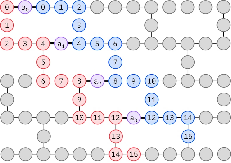
D'IBM® Hardware hät e Heavy-Hex-Gitter-Qubit-Topologie, in welchem Fall mir e "Zickzack"-Muster verwende könne, des unde dargestellt isch. In dem Muster werde Orbitale mit demselbe Spin uf Qubits mit ener Linientopologie abgebildet (rote und blaue Kreise), und e Verbindung zwischen Orbitale unterschiedliche Spins isch a jedem 4. Raumorbital vorhande, wobei d'Verbindung durch en Ancilla-Qubit (violetti Kreise) ermöglicht wird. In dem Fall sind d'Indexbedingunge

$$\begin{align*} \mathbf{J}^{\alpha\alpha} &: \set{(p, p+1) \; , \; p = 0, \ldots, N-2} \\ \mathbf{J}^{\alpha\beta} &: \set{(p, p) \;, \; p = 0, 4, 8, \ldots (p \leq N-1)} \end{align*}$$

Selbstkonsistente Konfigurationswiederherstellung

Des selbstkonsistente Konfigurationswiederherstellungsverfahre isch dazu ausgelegt, so viel Signal wie möglich us verrauschte Quantenstichproben ruszhole. Da de molekulare Hamiltonian d'Teilchenzahl und Spin-Z erhält, isch's sinnvoll, en Schaltkreis-Ansatz z'wähle, de disi Symmetriene au erhält. Wenn er uf de Hartree-Fock-Zustand a'g'wendet wird, hät de resultierend Zustand im rauschfreie Fall e festi Teilchenzahl und Spin-Z. Daher sollte d'Spin-$\alpha$- und d'Spin-$\beta$-Hälften vun jedem us dem Zustand g'sampelte Bitstring dasselbe Hamming-Gewicht wie im Hartree-Fock-Zustand hän. Wege em Vorhandensein vun Rausche in aktuelle Quantenprozessore werde manche g'messene Bitstrings disi Eigenschaft verletze. E einfache Form de Postselektion würde disi Bitstrings verwerfe, aber des isch verschwenderisch, weil disi Bitstrings vielleicht no ebbis Signal enthält. Des selbstkonsistente Wiederherstellungsverfahre versucht, en Teil vun dem Signal in de Nachbearbeitung wiederherzustelle. Des Verfahre isch iterativ und brucht als Eingabe e Schätzung de durchschnittliche Besetzunge vun jedem Orbital im Grundzustand, die zuerst us de Rohstichproben berechnet wird. Des Verfahre wird in ener Schleife usgeführt, und jede Iteration hät d'folgende Schritt:

1. Für jeden Bitstring, de d'spezifizierte Symmetriene verletzt, flippe Se si Bits mit emm probabilistischen Verfahre, des dazu ausgelegt isch, de Bitstring näher a d'aktuelle Schätzung de durchschnittliche Orbitalbesetzunge z'bringe, um en neue Bitstring z'erhalte.
2. Sammle Se alli alte und neue Bitstrings, die d'Symmetriene erfülle, und entnehme Se Teilmenge vun ener im Voraus g'wählte feste Größe.
3. Für jede Teilmenge vun Bitstrings projiziere Se de Hamiltonian in de durch d'entsprechende Basisvektore aufgespannte Unterraum (luege Se in de vorige Abschnitt für e Beschreibung vun dene Basisvektore) und berechne Se e Grundzustandsschätzung vum projizierten Hamiltonian uf emm klassische Computer.
4. Aktualisiere Se d'Schätzung de durchschnittliche Orbitalbesetzunge mit de Grundzustandsschätzung mit de niedrigste Energie.

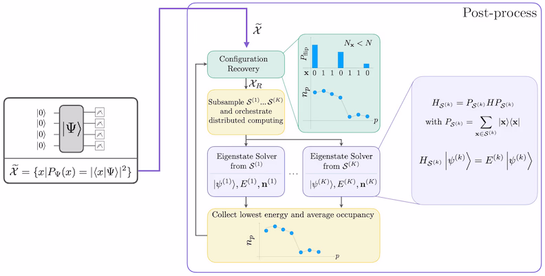
SQD-Workflow-Diagramm

De SQD-Workflow isch im folgende Diagramm dargestellt:

Anforderunge

Stellt Se vor em Beginne vun dem Tutorial sicher, dass Se Folgendes installiert hän:

• Qiskit SDK v1.0 oder höher, mit Visualisierungs-Unterstützung
• Qiskit Runtime v0.22 oder höher (pip install qiskit-ibm-runtime)
• SQD Qiskit Addon v0.11 oder höher (pip install qiskit-addon-sqd)
• ffsim v0.0.58 oder höher (pip install ffsim)

Setup

# Added by doQumentation — installs packages not in the Binder environment
!pip install -q ffsim qiskit-addon-sqd

import pyscf
import pyscf.cc
import pyscf.mcscf
import ffsim
import numpy as np
import matplotlib.pyplot as plt

from qiskit import QuantumCircuit, QuantumRegister
from qiskit.transpiler.preset_passmanagers import generate_preset_pass_manager

from qiskit_ibm_runtime import QiskitRuntimeService
from qiskit_ibm_runtime import SamplerV2 as Sampler

Schritt 1: Klassische Eingabe uf en Quantenproblem abbilden

In dem Tutorial finde mir e Approximation vum Grundzustand vum Molekül im Gleichgewicht im cc-pVDZ-Basissatz. Zuerst spezifiziere mir des Molekül und si Eigenschafte.

# Specify molecule properties
open_shell = False
spin_sq = 0

# Build N2 molecule
mol = pyscf.gto.Mole()
mol.build(
    atom=[["N", (0, 0, 0)], ["N", (1.0, 0, 0)]],
    basis="cc-pvdz",
    symmetry="Dooh",
)

# Define active space
n_frozen = 2
active_space = range(n_frozen, mol.nao_nr())

# Get molecular integrals
scf = pyscf.scf.RHF(mol).run()
num_orbitals = len(active_space)
n_electrons = int(sum(scf.mo_occ[active_space]))
num_elec_a = (n_electrons + mol.spin) // 2
num_elec_b = (n_electrons - mol.spin) // 2
cas = pyscf.mcscf.CASCI(scf, num_orbitals, (num_elec_a, num_elec_b))
mo = cas.sort_mo(active_space, base=0)
hcore, nuclear_repulsion_energy = cas.get_h1cas(mo)
eri = pyscf.ao2mo.restore(1, cas.get_h2cas(mo), num_orbitals)

# Store reference energy from SCI calculation performed separately
exact_energy = -109.22690201485733

converged SCF energy = -108.929838385609

Vor em Konstruiere vum LUCJ-Ansatz-Schaltkreis führe mir zunächst e CCSD-Berechnung in de folgende Code-Zelle durch. D' $t_1$- und $t_2$-Amplituden us dere Berechnung werde verwendet, um d'Parameter vum Ansatz z'initialisiere.

# Get CCSD t2 amplitudes for initializing the ansatz
ccsd = pyscf.cc.CCSD(
    scf, frozen=[i for i in range(mol.nao_nr()) if i not in active_space]
).run()
t1 = ccsd.t1
t2 = ccsd.t2

E(CCSD) = -109.2177884185543  E_corr = -0.2879500329450045

Jetzt verwende mir ffsim, um de Ansatz-Schaltkreis z'erstelle. Da unser Molekül en geschlosseschalige Hartree-Fock-Zustand hät, verwende mir d'spin-balancierte Variante vum UCJ-Ansatz, UCJOpSpinBalanced. Mir übergebe Wechselwirkungspaare, die für e Heavy-Hex-Gitter-Qubit-Topologie geeignet sind (luege Se in de Hintergrundabschnitt zum LUCJ-Ansatz). Mir setze optimize=True in de from_t_amplitudes-Methode, um d'"komprimierte" Doppelfaktorisierung de $t_2$-Amplituden z'ermögliche (luege Se The local unitary cluster Jastrow (LUCJ) ansatz in de ffsim-Dokumentation für Details).

n_reps = 1
alpha_alpha_indices = [(p, p + 1) for p in range(num_orbitals - 1)]
alpha_beta_indices = [(p, p) for p in range(0, num_orbitals, 4)]

ucj_op = ffsim.UCJOpSpinBalanced.from_t_amplitudes(
    t2=t2,
    t1=t1,
    n_reps=n_reps,
    interaction_pairs=(alpha_alpha_indices, alpha_beta_indices),
    # Setting optimize=True enables the "compressed" factorization
    optimize=True,
    # Limit the number of optimization iterations to prevent the code cell from running
    # too long. Removing this line may improve results.
    options=dict(maxiter=1000),
)

nelec = (num_elec_a, num_elec_b)

# create an empty quantum circuit
qubits = QuantumRegister(2 * num_orbitals, name="q")
circuit = QuantumCircuit(qubits)

# prepare Hartree-Fock state as the reference state and append it to the quantum circuit
circuit.append(ffsim.qiskit.PrepareHartreeFockJW(num_orbitals, nelec), qubits)

# apply the UCJ operator to the reference state
circuit.append(ffsim.qiskit.UCJOpSpinBalancedJW(ucj_op), qubits)
circuit.measure_all()

Schritt 2: Problem für Quantenhardware-Ausführung optimiere

Als Nächstes optimiere mir de Schaltkreis für e Ziel-Hardware.

service = QiskitRuntimeService()
backend = service.least_busy(
    operational=True, simulator=False, min_num_qubits=133
)

print(f"Using backend {backend.name}")

Using backend ibm_fez

Mir empfehle d'folgende Schritt, um de Ansatz z'optimiere und hardware-kompatibel z'mache.

• Wähle Se physikalische Qubits (initial_layout) us de Ziel-Hardware us, die em zuvor beschriebene "Zickzack"-Muster entspreche. Des Anlege vun Qubits in dem Muster führt zu emm effizienten hardware-kompatible Schaltkreis mit weniger Gates. Do füge mir Code i, um d'Auswahl vum "Zickzack"-Muster z'automatisiere, de e Bewertungsheuristik verwendet, um d'mit em ausgewählte Layout verbundene Fehler z'minimiere.
• Generiere Se en gestuften Pass-Manager mit de Funktion generate_preset_pass_manager vun Qiskit mit Ihrer Wahl vun backend und initial_layout.
• Setze Se d' pre_init-Stufe vun Ihrem gestuften Pass-Manager uf ffsim.qiskit.PRE_INIT. ffsim.qiskit.PRE_INIT enthält Qiskit-Transpiler-Pässe, die Gates in Orbitalrotationen zerleget und dann d'Orbitalrotationen zusammenführet, was zu weniger Gates im endgültige Schaltkreis führt.
• Führe Se de Pass-Manager uf Ihrem Schaltkreis us.

Code für automatisierte Auswahl vum "Zickzack"-Layout

from typing import Sequence

import rustworkx
from qiskit.providers import BackendV2
from rustworkx import NoEdgeBetweenNodes, PyGraph

IBM_TWO_Q_GATES = {"cx", "ecr", "cz"}

def create_linear_chains(num_orbitals: int) -> PyGraph:
    """In zig-zag layout, there are two linear chains (with connecting qubits between
    the chains). This function creates those two linear chains: a rustworkx PyGraph
    with two disconnected linear chains. Each chain contains `num_orbitals` number
    of nodes, that is, in the final graph there are `2 * num_orbitals` number of nodes.

    Args:
        num_orbitals (int): Number orbitals or nodes in each linear chain. They are
            also known as alpha-alpha interaction qubits.

    Returns:
        A rustworkx.PyGraph with two disconnected linear chains each with `num_orbitals`
            number of nodes.
    """
    G = rustworkx.PyGraph()

    for n in range(num_orbitals):
        G.add_node(n)

    for n in range(num_orbitals - 1):
        G.add_edge(n, n + 1, None)

    for n in range(num_orbitals, 2 * num_orbitals):
        G.add_node(n)

    for n in range(num_orbitals, 2 * num_orbitals - 1):
        G.add_edge(n, n + 1, None)

    return G

def create_lucj_zigzag_layout(
    num_orbitals: int, backend_coupling_graph: PyGraph
) -> tuple[PyGraph, int]:
    """This function creates the complete zigzag graph that 'can be mapped' to an IBM QPU with
    heavy-hex connectivity (the zigzag must be an isomorphic sub-graph to the QPU/backend
    coupling graph for it to be mapped).
    The zigzag pattern includes both linear chains (alpha-alpha interactions) and connecting
    qubits between the linear chains (alpha-beta interactions).

    Args:
        num_orbitals (int): Number of orbitals, that is, number of nodes in each alpha-alpha linear chain.
        backend_coupling_graph (PyGraph): The coupling graph of the backend on which the LUCJ ansatz
            will be mapped and run. This function takes the coupling graph as a undirected
            `rustworkx.PyGraph` where there is only one 'undirected' edge between two nodes,
            that is, qubits. Usually, the coupling graph of a IBM backend is directed (for example, Eagle devices
            such as ibm_brisbane) or may have two edges between two nodes (for example, Heron `ibm_torino`).
            A user needs to be make such graphs undirected and/or remove duplicate edges to make them
            compatible with this function.

    Returns:
        G_new (PyGraph): The graph with IBM backend compliant zigzag pattern.
        num_alpha_beta_qubits (int): Number of connecting qubits between the linear chains
            in the zigzag pattern. While we want as many connecting (alpha-beta) qubits between
            the linear (alpha-alpha) chains, we cannot accommodate all due to qubit and connectivity
            constraints of backends. This is the maximum number of connecting qubits the zigzag pattern
            can have while being backend compliant (that is, isomorphic to backend coupling graph).
    """
    isomorphic = False
    G = create_linear_chains(num_orbitals=num_orbitals)

    num_iters = num_orbitals
    while not isomorphic:
        G_new = G.copy()
        num_alpha_beta_qubits = 0
        for n in range(num_iters):
            if n % 4 == 0:
                new_node = 2 * num_orbitals + num_alpha_beta_qubits
                G_new.add_node(new_node)
                G_new.add_edge(n, new_node, None)
                G_new.add_edge(new_node, n + num_orbitals, None)
                num_alpha_beta_qubits = num_alpha_beta_qubits + 1
        isomorphic = rustworkx.is_subgraph_isomorphic(
            backend_coupling_graph, G_new
        )
        num_iters -= 1

    return G_new, num_alpha_beta_qubits

def lightweight_layout_error_scoring(
    backend: BackendV2,
    virtual_edges: Sequence[Sequence[int]],
    physical_layouts: Sequence[int],
    two_q_gate_name: str,
) -> list[list[list[int], float]]:
    """Lightweight and heuristic function to score isomorphic layouts. There can be many zigzag patterns,
    each with different set of physical qubits, that can be mapped to a backend. Some of them may
    include less noise qubits and couplings than others. This function computes a simple error score
    for each such layout. It sums up 2Q gate error for all couplings in the zigzag pattern (layout) and
    measurement of errors of physical qubits in the layout to compute the error score.

    Note:
        This lightweight scoring can be refined using concepts such as mapomatic.

    Args:
        backend (BackendV2): A backend.
        virtual_edges (Sequence[Sequence[int]]): Edges in the device compliant zigzag pattern where
            nodes are numbered from 0 to (2 * num_orbitals + num_alpha_beta_qubits).
        physical_layouts (Sequence[int]): All physical layouts of the zigzag pattern that are isomorphic
            to each other and to the larger backend coupling map.
        two_q_gate_name (str): The name of the two-qubit gate of the backend. The name is used for fetching
            two-qubit gate error from backend properties.

    Returns:
        scores (list): A list of lists where each sublist contains two items. First item is the layout, and
            second item is a float representing error score of the layout. The layouts in the `scores` are
            sorted in the ascending order of error score.
    """
    props = backend.properties()
    scores = []
    for layout in physical_layouts:
        total_2q_error = 0
        for edge in virtual_edges:
            physical_edge = (layout[edge[0]], layout[edge[1]])
            try:
                ge = props.gate_error(two_q_gate_name, physical_edge)
            except Exception:
                ge = props.gate_error(two_q_gate_name, physical_edge[::-1])
            total_2q_error += ge
        total_measurement_error = 0
        for qubit in layout:
            meas_error = props.readout_error(qubit)
            total_measurement_error += meas_error
        scores.append([layout, total_2q_error + total_measurement_error])

    return sorted(scores, key=lambda x: x[1])

def _make_backend_cmap_pygraph(backend: BackendV2) -> PyGraph:
    graph = backend.coupling_map.graph
    if not graph.is_symmetric():
        graph.make_symmetric()
    backend_coupling_graph = graph.to_undirected()

    edge_list = backend_coupling_graph.edge_list()
    removed_edge = []
    for edge in edge_list:
        if set(edge) in removed_edge:
            continue
        try:
            backend_coupling_graph.remove_edge(edge[0], edge[1])
            removed_edge.append(set(edge))
        except NoEdgeBetweenNodes:
            pass

    return backend_coupling_graph

def get_zigzag_physical_layout(
    num_orbitals: int, backend: BackendV2, score_layouts: bool = True
) -> tuple[list[int], int]:
    """The main function that generates the zigzag pattern with physical qubits that can be used
    as an `intial_layout` in a preset passmanager/transpiler.

    Args:
        num_orbitals (int): Number of orbitals.
        backend (BackendV2): A backend.
        score_layouts (bool): Optional. If `True`, it uses the `lightweight_layout_error_scoring`
            function to score the isomorphic layouts and returns the layout with less erroneous qubits.
            If `False`, returns the first isomorphic subgraph.

    Returns:
        A tuple of device compliant layout (list[int]) with zigzag pattern and an int representing
            number of alpha-beta-interactions.
    """
    backend_coupling_graph = _make_backend_cmap_pygraph(backend=backend)

    G, num_alpha_beta_qubits = create_lucj_zigzag_layout(
        num_orbitals=num_orbitals,
        backend_coupling_graph=backend_coupling_graph,
    )

    isomorphic_mappings = rustworkx.vf2_mapping(
        backend_coupling_graph, G, subgraph=True
    )
    isomorphic_mappings = list(isomorphic_mappings)

    edges = list(G.edge_list())

    layouts = []
    for mapping in isomorphic_mappings:
        initial_layout = [None] * (2 * num_orbitals + num_alpha_beta_qubits)
        for key, value in mapping.items():
            initial_layout[value] = key
        layouts.append(initial_layout)

    two_q_gate_name = IBM_TWO_Q_GATES.intersection(
        backend.configuration().basis_gates
    ).pop()

    if score_layouts:
        scores = lightweight_layout_error_scoring(
            backend=backend,
            virtual_edges=edges,
            physical_layouts=layouts,
            two_q_gate_name=two_q_gate_name,
        )

        return scores[0][0][:-num_alpha_beta_qubits], num_alpha_beta_qubits

    return layouts[0][:-num_alpha_beta_qubits], num_alpha_beta_qubits

initial_layout, _ = get_zigzag_physical_layout(num_orbitals, backend=backend)

pass_manager = generate_preset_pass_manager(
    optimization_level=3, backend=backend, initial_layout=initial_layout
)

# without PRE_INIT passes
 isa_circuit = pass_manager.run(circuit)
print(f"Gate counts (w/o pre-init passes): {isa_circuit.count_ops()}")

# with PRE_INIT passes
# We will use the circuit generated by this pass manager for hardware execution
pass_manager.pre_init = ffsim.qiskit.PRE_INIT
 isa_circuit = pass_manager.run(circuit)
print(f"Gate counts (w/ pre-init passes): {isa_circuit.count_ops()}")

Gate counts (w/o pre-init passes): OrderedDict({'rz': 12438, 'sx': 12169, 'cz': 3986, 'x': 573, 'measure': 52, 'barrier': 1})
Gate counts (w/ pre-init passes): OrderedDict({'sx': 7059, 'rz': 6962, 'cz': 1876, 'measure': 52, 'x': 35, 'barrier': 1})

Schritt 3: Usführe mit Qiskit-Primitive

Nach de Optimierung vum Schaltkreis für d'Hardware-Ausführung sind mir bereit, ihn uf de Ziel-Hardware usz'führe und Stichproben für d'Grundzustandsenergieabschätzung z'sammle. Da mir nur en Schaltkreis hän, verwende mir de Job-Ausführungsmodus vun Qiskit Runtime und führe unsere Schaltkreis us.

sampler = Sampler(mode=backend)
job = sampler.run([isa_circuit], shots=100_000)

primitive_result = job.result()
pub_result = primitive_result[0]

Schritt 4: Nachbearbeitung und Rückgabe vum Ergebnis im g'wünschte klassische Format

Jetzt schätze mir d'Grundzustandsenergie vum Hamiltonian mit de Funktion diagonalize_fermionic_hamiltonian. Disi Funktion führt des selbstkonsistente Konfigurationswiederherstellungsverfahre us, um d'verrauschte Quantenstichproben iterativ z'verfeinere und d'Energieabschätzung z'verbessere. Mir übergebe e Callback-Funktion, damit mir d'Zwischenergebnisse für e spätere Analyse speichere könne. Luege Se in d' API-Dokumentation für Erklärunge de Argumente vun diagonalize_fermionic_hamiltonian.

from functools import partial

from qiskit_addon_sqd.fermion import (
    SCIResult,
    diagonalize_fermionic_hamiltonian,
    solve_sci_batch,
)

# SQD options
energy_tol = 1e-3
occupancies_tol = 1e-3
max_iterations = 5

# Eigenstate solver options
num_batches = 3
samples_per_batch = 300
symmetrize_spin = True
carryover_threshold = 1e-4
max_cycle = 200

# Pass options to the built-in eigensolver. If you just want to use the defaults,
# you can omit this step, in which case you would not specify the sci_solver argument
# in the call to diagonalize_fermionic_hamiltonian below.
sci_solver = partial(solve_sci_batch, spin_sq=0.0, max_cycle=max_cycle)

# List to capture intermediate results
result_history = []

def callback(results: list[SCIResult]):
    result_history.append(results)
    iteration = len(result_history)
    print(f"Iteration {iteration}")
    for i, result in enumerate(results):
        print(f"\tSubsample {i}")
        print(f"\t\tEnergy: {result.energy + nuclear_repulsion_energy}")
        print(
            f"\t\tSubspace dimension: {np.prod(result.sci_state.amplitudes.shape)}"
        )

result = diagonalize_fermionic_hamiltonian(
    hcore,
    eri,
    pub_result.data.meas,
    samples_per_batch=samples_per_batch,
    norb=num_orbitals,
    nelec=nelec,
    num_batches=num_batches,
    energy_tol=energy_tol,
    occupancies_tol=occupancies_tol,
    max_iterations=max_iterations,
    sci_solver=sci_solver,
    symmetrize_spin=symmetrize_spin,
    carryover_threshold=carryover_threshold,
    callback=callback,
    seed=12345,
)

Iteration 1
	Subsample 0
		Energy: -108.97781410104506
		Subspace dimension: 28561
	Subsample 1
		Energy: -108.97781410104506
		Subspace dimension: 28561
	Subsample 2
		Energy: -108.97781410104506
		Subspace dimension: 28561
Iteration 2
	Subsample 0
		Energy: -109.05150860754739
		Subspace dimension: 287296
	Subsample 1
		Energy: -109.08152283263908
		Subspace dimension: 264196
	Subsample 2
		Energy: -109.11636893067873
		Subspace dimension: 284089
Iteration 3
	Subsample 0
		Energy: -109.15878555367885
		Subspace dimension: 429025
	Subsample 1
		Energy: -109.16462831275786
		Subspace dimension: 473344
	Subsample 2
		Energy: -109.15895026995382
		Subspace dimension: 435600
Iteration 4
	Subsample 0
		Energy: -109.17784051223317
		Subspace dimension: 622521
	Subsample 1
		Energy: -109.1774651326829
		Subspace dimension: 657721
	Subsample 2
		Energy: -109.18085212360191
		Subspace dimension: 617796
Iteration 5
	Subsample 0
		Energy: -109.18636242518915
		Subspace dimension: 815409
	Subsample 1
		Energy: -109.18451014767518
		Subspace dimension: 837225
	Subsample 2
		Energy: -109.18333728638888
		Subspace dimension: 857476

Visualisierung de Ergebnisse

De erste Plot zeigt, dass mir nach e paar Iterationen d'Grundzustandsenergie innerhalb vun ~41 mH schätze (chemische Genauigkeit wird typischerweise als 1 kcal/mol $\approx$ 1.6 mH akzeptiert). D'Energie ka verbessert werde, indem mehr Iterationen de Konfigurationswiederherstellung erlaubt werde oder d'Anzahl de Stichproben pro Batch erhöht wird.

De zweite Plot zeigt d'durchschnittliche Besetzung vun jedem Raumorbital nach de letzte Iteration. Mir könne sehe, dass sowohl d'Spin-Up- als au d'Spin-Down-Elektronen d'erste fünf Orbitale mit hoher Wahrscheinlichkeit in unsere Lösungen besetze.

# Data for energies plot
x1 = range(len(result_history))
min_e = [
    min(result, key=lambda res: res.energy).energy + nuclear_repulsion_energy
    for result in result_history
]
e_diff = [abs(e - exact_energy) for e in min_e]
yt1 = [1.0, 1e-1, 1e-2, 1e-3, 1e-4]

# Chemical accuracy (+/- 1 milli-Hartree)
chem_accuracy = 0.001

# Data for avg spatial orbital occupancy
y2 = np.sum(result.orbital_occupancies, axis=0)
x2 = range(len(y2))

fig, axs = plt.subplots(1, 2, figsize=(12, 6))

# Plot energies
axs[0].plot(x1, e_diff, label="energy error", marker="o")
axs[0].set_xticks(x1)
axs[0].set_xticklabels(x1)
axs[0].set_yticks(yt1)
axs[0].set_yticklabels(yt1)
axs[0].set_yscale("log")
axs[0].set_ylim(1e-4)
axs[0].axhline(
    y=chem_accuracy,
    color="#BF5700",
    linestyle="--",
    label="chemical accuracy",
)
axs[0].set_title("Approximated Ground State Energy Error vs SQD Iterations")
axs[0].set_xlabel("Iteration Index", fontdict={"fontsize": 12})
axs[0].set_ylabel("Energy Error (Ha)", fontdict={"fontsize": 12})
axs[0].legend()

# Plot orbital occupancy
axs[1].bar(x2, y2, width=0.8)
axs[1].set_xticks(x2)
axs[1].set_xticklabels(x2)
axs[1].set_title("Avg Occupancy per Spatial Orbital")
axs[1].set_xlabel("Orbital Index", fontdict={"fontsize": 12})
axs[1].set_ylabel("Avg Occupancy", fontdict={"fontsize": 12})

plt.tight_layout()
plt.show()

Tutorial-Umfrage

Bitte nehme Se a dere kurze Umfrage teil, um Feedback zu dem Tutorial z'gebe. Ihri Einblicke helfe uns, unseri Inhaltsangebote und Benutzererfahrung z'verbessere.

Link zur Umfrage