Pauli-Korrelations-Encoding zur Verkleinerung vo de Maxcut-Aafordrige

Nutzungsschätzung: 30 Minüte uf emem Eagle r3 Prozessor (HINWEIS: Des isch nit meh als e Schätzung. Iri Laufzeit ka variiere.)

Hintergrund

Des Tutorial stellt Pauli-Korrelations-Encoding (PCE) [1] vor, en Aasatz zur effizienter Kodierung vo Optimierungsprobleme in Qubits für Quanteberechnige. PCE bildet klassischi Variabli in Optimierungsprobleme uf Mehrkörper-Pauli-Matrix-Korrelationä ab, was zu enere polynomielle Kompression vo de Platzaafordrige vom Problem führt. Durch de Einsatz vo PCE wird d'Aazahl vo de für d'Kodierung benötigte Qubits verkleinert, was besonders vorteilhaft isch für kurzfristigi Quantegerät mit begrenzti Qubit-Ressourcä. Dazu isch analytisch nochgwise, dass PCE inhärent Barren Plateaus abschwächt und super-polynomielle Widerstandsfähigkeit gege des Phänomen bietet. Des igbaute Eigenschaft ermöglicht beischwellose Leistig bei Quante-Optimierungslöser.

Überblick

De PCE-Aasatz besteht us drei Hauptschritt, wie in Abbildig 1 us [1] unne dargestellt isch:

1. Kodierung vom Optimierungsproblem in en Pauli-Korrelationsraum.
2. Lösung vom Problem mit emem quante-klassische Optimierungslöser.
3. Dekodierung vo de Lösung zruck in de ursprünglich Optimierungsraum. De PCE-Aasatz isch aapsbar an jeden Quante-Optimierungslöser, de Pauli-Korrelationsmatrize verarbeite ka. 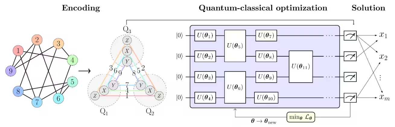In Abbildig 1 us [1] wird des Max-Cut-Problem als Beispiel zur Veranschaulichig vom PCE-Aasatz verwendet. Des Max-Cut-Problem mit $m=9$ Knote wird in en Pauli-Korrelationsraum kodiert, wobei des Optimierungsproblem als Korrelationsmatrix dargestellt wird, insbesondere als 2-Körper-Pauli-Matrix-Korrelationä über $n=3$ Qubits $(Q_1, Q_2, Q_3)$. Knotefarbe gänd de Pauli-String aa, de für jeden kodiierte Knote verwendet wird. Zum Beispiel wird Knote 1, de de binäri Variabli $x_1$ entspricht, durch de Erwartungswert vo $Z_1 \otimes Z_2 \otimes I_3$ kodiert, während $x_8$ durch $I_1 \otimes Y_2 \otimes Y_3$ kodiert wird. Des entspricht enere Kompression vo de $m$ Variabli vom Problem in $n = O(m^{1/2})$ Qubits. Allgemener ermöglicht $k$-Körper-Korrelationä polynomielle Kompressione vo de Ordnig $k$. De gwählte Pauli-Satz umfasst drei Teilmenge vo gegaseitig kommutierendi Pauli-Strings, wodurch alli $m$ Korrelationä experimentell mit nit meh als drei Messeinstellige gschätzt werre könne.

En Verlustfunktion $\mathcal{L}$ vo Pauli-Erwartungswerte, die d'ursprünglich Max-Cut-Zielfunktion nachahmt, wird konstruiert. D'Verlustfunktion wird dann mit emem quante-klassische Optimierungslöser wie dem Variational Quantum Eigensolver (VQE) optimiert.

Sobald d'Optimierig abgschlosse isch, wird d'Lösung in de ursprünglich Optimierungsraum zurückdekodiert, wodurch d'optimal Max-Cut-Lösung erhalt wird.

Aafordrige

Stellt vor em Aafang vo dem Tutorial sicher, dass mir des Folgende installiert hän:

• Qiskit SDK v1.0 oder höher, mit Visualisierungs-Unterstützung
• Qiskit Runtime v0.22 oder höher (pip install qiskit-ibm-runtime)

Irichtig

# Added by doQumentation — installs packages not in the Binder environment
!pip install -q networkx

from itertools import combinations

import numpy as np
import rustworkx as rx
from scipy.optimize import minimize

from qiskit.circuit.library import efficient_su2
from qiskit.transpiler.preset_passmanagers import generate_preset_pass_manager
from qiskit.quantum_info import SparsePauliOp
from qiskit_ibm_runtime import EstimatorV2 as Estimator
from qiskit_ibm_runtime import QiskitRuntimeService
from qiskit_ibm_runtime import Session
from rustworkx.visualization import mpl_draw

service = QiskitRuntimeService()
backend = service.least_busy(
    operational=True, simulator=False, min_num_qubits=127
)

def calc_cut_size(graph, partition0, partition1):
    """Calculate the cut size of the given partitions of the graph."""

    cut_size = 0
    for edge0, edge1 in graph.edge_list():
        if edge0 in partition0 and edge1 in partition1:
            cut_size += 1
        elif edge0 in partition1 and edge1 in partition0:
            cut_size += 1
    return cut_size

Schritt 1: Klassischi Igabe uf as Quanteproblem aabilde

Max-Cut-Problem

Des Max-Cut-Problem isch en kombinatorisches Optimierungsproblem, des uf emem Graphe $G = (V, E)$ definiert isch, wobei $V$ d'Menge vo de Knote und $E$ d'Menge vo de Kante isch. Des Ziel isch, d'Knote in zwoi Menge $S$ und $V \setminus S$ z'partitioniere, sodass d'Aazahl vo de Kante zwische de zwoi Menge maximiert wird. Für en ausführlicheri Beschribig vom Max-Cut-Problem verwised bitte uf des Tutorial "Quantum approximate optimization algorithm". Außerdem wird des Max-Cut-Problem als Beispiel im Tutorial "Advanced Techniques for QAOA" verwendet. In dene Tutorials wird de QAOA-Algorithmus zur Lösung vom Max-Cut-Problem igsetzt.

Graph -> Hamiltonian

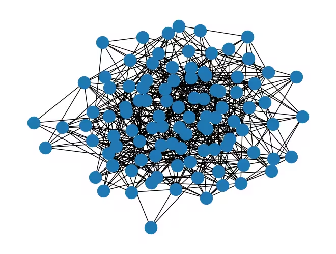
Des Tutorial verwendet en Zufallsgraph mit 1000 Knote.

D'Problemgröße isch möglicherwis schwer z'visualisiere, deshalb isch unne en Graph mit 100 Knote dargestellt. (D'direkt Darstellig vo emem Graphe mit 1.000 Knote würd'n zu dicht mache, um öppis z'sehe!) De Graph, mit dem mir arbete, isch zehnmal größer.

mpl_draw(rx.undirected_gnp_random_graph(100, 0.1, seed=42))

num_nodes = 1000  # Number of nodes in graph
graph = rx.undirected_gnp_random_graph(num_nodes, 0.1, seed=42)

import networkx as nx

nx_graph = nx.Graph()
nx_graph.add_nodes_from(range(num_nodes))

for edge in graph.edge_list():
    nx_graph.add_edge(edge[0], edge[1])

curr_cut_size, partition = nx.approximation.one_exchange(nx_graph, seed=1)
print(f"Initial cut size: {curr_cut_size}")

Initial cut size: 28075

Mir kodiered de Graph mit 1000 Knote in 2-Körper-Pauli-Matrix-Korrelationä über 100 Qubits. De Graph wird als Korrelationsmatrix dargestellt, wobei jeder Knote durch en Pauli-String kodiert wird. Des Vorzeiche vom Erwartungswert vom Pauli-String gibt d'Partition vom Knote aa. Zum Beispiel wird Knote 0 durch en Pauli-String kodiert, $\prod_0 = I_{19} \otimes ... I_2 \otimes X_1 \otimes X_0$. Des Vorzeiche vom Erwartungswert vo dem Pauli-String gibt d'Partition vo Knote 0 aa. Mir definiered en Pauli-Korrelations-Encoding (PCE) relativ zu $\prod$ als

$x_i \coloneqq \textit{sgn}(\langle\prod_i \rangle)$

wobei $x_i$ d'Partition vo Knote $i$ isch und $\langle \prod_i \rangle \coloneqq \langle \psi |\prod_i| \psi \rangle$ de Erwartungswert vom Pauli-String isch, de Knote $i$ über en Quantezustand $|\psi \rangle$ kodiert. Jetzt kodiered mir de Graph mit PCE in en Hamiltonian. Mir teiled d'Knote in drei Menge uf: $S_1$, $S_2$ und $S_3$. Dann kodiered mir d'Knote in jedere Menge mit de Pauli-Strings $X$, $Y$ bzw. $Z$.

num_qubits = 100

list_size = num_nodes // 3
node_x = [i for i in range(list_size)]
node_y = [i for i in range(list_size, 2 * list_size)]
node_z = [i for i in range(2 * list_size, num_nodes)]

print("List 1:", node_x)
print("List 2:", node_y)
print("List 3:", node_z)

List 1: [0, 1, 2, 3, 4, 5, 6, 7, 8, 9, 10, 11, 12, 13, 14, 15, 16, 17, 18, 19, 20, 21, 22, 23, 24, 25, 26, 27, 28, 29, 30, 31, 32, 33, 34, 35, 36, 37, 38, 39, 40, 41, 42, 43, 44, 45, 46, 47, 48, 49, 50, 51, 52, 53, 54, 55, 56, 57, 58, 59, 60, 61, 62, 63, 64, 65, 66, 67, 68, 69, 70, 71, 72, 73, 74, 75, 76, 77, 78, 79, 80, 81, 82, 83, 84, 85, 86, 87, 88, 89, 90, 91, 92, 93, 94, 95, 96, 97, 98, 99, 100, 101, 102, 103, 104, 105, 106, 107, 108, 109, 110, 111, 112, 113, 114, 115, 116, 117, 118, 119, 120, 121, 122, 123, 124, 125, 126, 127, 128, 129, 130, 131, 132, 133, 134, 135, 136, 137, 138, 139, 140, 141, 142, 143, 144, 145, 146, 147, 148, 149, 150, 151, 152, 153, 154, 155, 156, 157, 158, 159, 160, 161, 162, 163, 164, 165, 166, 167, 168, 169, 170, 171, 172, 173, 174, 175, 176, 177, 178, 179, 180, 181, 182, 183, 184, 185, 186, 187, 188, 189, 190, 191, 192, 193, 194, 195, 196, 197, 198, 199, 200, 201, 202, 203, 204, 205, 206, 207, 208, 209, 210, 211, 212, 213, 214, 215, 216, 217, 218, 219, 220, 221, 222, 223, 224, 225, 226, 227, 228, 229, 230, 231, 232, 233, 234, 235, 236, 237, 238, 239, 240, 241, 242, 243, 244, 245, 246, 247, 248, 249, 250, 251, 252, 253, 254, 255, 256, 257, 258, 259, 260, 261, 262, 263, 264, 265, 266, 267, 268, 269, 270, 271, 272, 273, 274, 275, 276, 277, 278, 279, 280, 281, 282, 283, 284, 285, 286, 287, 288, 289, 290, 291, 292, 293, 294, 295, 296, 297, 298, 299, 300, 301, 302, 303, 304, 305, 306, 307, 308, 309, 310, 311, 312, 313, 314, 315, 316, 317, 318, 319, 320, 321, 322, 323, 324, 325, 326, 327, 328, 329, 330, 331, 332]
List 2: [333, 334, 335, 336, 337, 338, 339, 340, 341, 342, 343, 344, 345, 346, 347, 348, 349, 350, 351, 352, 353, 354, 355, 356, 357, 358, 359, 360, 361, 362, 363, 364, 365, 366, 367, 368, 369, 370, 371, 372, 373, 374, 375, 376, 377, 378, 379, 380, 381, 382, 383, 384, 385, 386, 387, 388, 389, 390, 391, 392, 393, 394, 395, 396, 397, 398, 399, 400, 401, 402, 403, 404, 405, 406, 407, 408, 409, 410, 411, 412, 413, 414, 415, 416, 417, 418, 419, 420, 421, 422, 423, 424, 425, 426, 427, 428, 429, 430, 431, 432, 433, 434, 435, 436, 437, 438, 439, 440, 441, 442, 443, 444, 445, 446, 447, 448, 449, 450, 451, 452, 453, 454, 455, 456, 457, 458, 459, 460, 461, 462, 463, 464, 465, 466, 467, 468, 469, 470, 471, 472, 473, 474, 475, 476, 477, 478, 479, 480, 481, 482, 483, 484, 485, 486, 487, 488, 489, 490, 491, 492, 493, 494, 495, 496, 497, 498, 499, 500, 501, 502, 503, 504, 505, 506, 507, 508, 509, 510, 511, 512, 513, 514, 515, 516, 517, 518, 519, 520, 521, 522, 523, 524, 525, 526, 527, 528, 529, 530, 531, 532, 533, 534, 535, 536, 537, 538, 539, 540, 541, 542, 543, 544, 545, 546, 547, 548, 549, 550, 551, 552, 553, 554, 555, 556, 557, 558, 559, 560, 561, 562, 563, 564, 565, 566, 567, 568, 569, 570, 571, 572, 573, 574, 575, 576, 577, 578, 579, 580, 581, 582, 583, 584, 585, 586, 587, 588, 589, 590, 591, 592, 593, 594, 595, 596, 597, 598, 599, 600, 601, 602, 603, 604, 605, 606, 607, 608, 609, 610, 611, 612, 613, 614, 615, 616, 617, 618, 619, 620, 621, 622, 623, 624, 625, 626, 627, 628, 629, 630, 631, 632, 633, 634, 635, 636, 637, 638, 639, 640, 641, 642, 643, 644, 645, 646, 647, 648, 649, 650, 651, 652, 653, 654, 655, 656, 657, 658, 659, 660, 661, 662, 663, 664, 665]
List 3: [666, 667, 668, 669, 670, 671, 672, 673, 674, 675, 676, 677, 678, 679, 680, 681, 682, 683, 684, 685, 686, 687, 688, 689, 690, 691, 692, 693, 694, 695, 696, 697, 698, 699, 700, 701, 702, 703, 704, 705, 706, 707, 708, 709, 710, 711, 712, 713, 714, 715, 716, 717, 718, 719, 720, 721, 722, 723, 724, 725, 726, 727, 728, 729, 730, 731, 732, 733, 734, 735, 736, 737, 738, 739, 740, 741, 742, 743, 744, 745, 746, 747, 748, 749, 750, 751, 752, 753, 754, 755, 756, 757, 758, 759, 760, 761, 762, 763, 764, 765, 766, 767, 768, 769, 770, 771, 772, 773, 774, 775, 776, 777, 778, 779, 780, 781, 782, 783, 784, 785, 786, 787, 788, 789, 790, 791, 792, 793, 794, 795, 796, 797, 798, 799, 800, 801, 802, 803, 804, 805, 806, 807, 808, 809, 810, 811, 812, 813, 814, 815, 816, 817, 818, 819, 820, 821, 822, 823, 824, 825, 826, 827, 828, 829, 830, 831, 832, 833, 834, 835, 836, 837, 838, 839, 840, 841, 842, 843, 844, 845, 846, 847, 848, 849, 850, 851, 852, 853, 854, 855, 856, 857, 858, 859, 860, 861, 862, 863, 864, 865, 866, 867, 868, 869, 870, 871, 872, 873, 874, 875, 876, 877, 878, 879, 880, 881, 882, 883, 884, 885, 886, 887, 888, 889, 890, 891, 892, 893, 894, 895, 896, 897, 898, 899, 900, 901, 902, 903, 904, 905, 906, 907, 908, 909, 910, 911, 912, 913, 914, 915, 916, 917, 918, 919, 920, 921, 922, 923, 924, 925, 926, 927, 928, 929, 930, 931, 932, 933, 934, 935, 936, 937, 938, 939, 940, 941, 942, 943, 944, 945, 946, 947, 948, 949, 950, 951, 952, 953, 954, 955, 956, 957, 958, 959, 960, 961, 962, 963, 964, 965, 966, 967, 968, 969, 970, 971, 972, 973, 974, 975, 976, 977, 978, 979, 980, 981, 982, 983, 984, 985, 986, 987, 988, 989, 990, 991, 992, 993, 994, 995, 996, 997, 998, 999]

def build_pauli_correlation_encoding(pauli, node_list, n, k=2):
    pauli_correlation_encoding = []
    for idx, c in enumerate(combinations(range(n), k)):
        if idx >= len(node_list):
            break
        paulis = ["I"] * n
        paulis[c[0]], paulis[c[1]] = pauli, pauli
        pauli_correlation_encoding.append(("".join(paulis)[::-1], 1))

    hamiltonian = []
    for pauli, weight in pauli_correlation_encoding:
        hamiltonian.append(SparsePauliOp.from_list([(pauli, weight)]))

    return hamiltonian

pauli_correlation_encoding_x = build_pauli_correlation_encoding(
    "X", node_x, num_qubits
)
pauli_correlation_encoding_y = build_pauli_correlation_encoding(
    "Y", node_y, num_qubits
)
pauli_correlation_encoding_z = build_pauli_correlation_encoding(
    "Z", node_z, num_qubits
)

Schritt 2: Problem für d'Usführig uf Quante-Hardware optimiere

Quanteschaltkreis

Do wird de Zustand $|\psi \rangle$ mit $\mathbf{\theta}$ parametrisiert, und mir optimiered deni Parameter $\mathbf{\theta}$ mit emem variationelle Aasatz. Des Tutorial verwendet de efficient_su2 Aasatz für unsere variationelle Algorithmus wege sinere Usdrucksfähigkeit und einfachene Implementierig. Mir verwended au d'relaxiert Verlustfunktion, die später in dem Tutorial iigeführt wird. Als Ergebnis könned mir großskalig Probleme mit weniger Qubits und geringeri Schaltkreistiefen aagehe.

# Build the quantum circuit
qc = efficient_su2(num_qubits, ["ry", "rz"], reps=2)

# Optimize the circuit

pm = generate_preset_pass_manager(optimization_level=3, backend=backend)
qc = pm.run(qc)

Verlustfunktion

Für d'Verlustfunktion $\mathcal{L}$ verwended mir en Relaxation vo de Max-Cut-Zielfunktion wie in [1] beschriewe, die als $\mathcal{V}(\mathbf{x}) \coloneqq \sum_{(i, j) \in E} W_{i, j}(1-x_i x_j)$ definiert isch. Do bezeichnet $W_{i, j}$ des Gewicht vo de Kante $(i, j)$ und $x_i$ d'Partition vo Knote $i$. D'Verlustfunktion $\mathcal{L}$ isch gebe durch:

$\mathcal{L}\coloneqq \sum_{(i, j) \in E} W_{i, j} \text{tanh} (\alpha \langle\prod_i \rangle) \text{tanh} (\alpha \langle\prod_j \rangle) + \mathcal{L}^{(\text{reg})}$

wobei d'Max-Cut-Zielfunktion durch glatti hyperbolischi Tangenti vo de Erwartungswerte vo de Pauli-Strings ersetzt wird, die d'Knote kodiered. De Regularisierungsterm $\mathcal{L}^{(\text{reg})}$ und de Skalierungsfaktor $\alpha$, proportional zur Aazahl vo de Qubits, werde iigeführt, um d'Leistig vom Löser z'verbessere.

De Regularisierungsterm isch definiert als:

$\mathcal{L}^{(\text{reg})}$ isch definiert als $\mathcal{L}^{(\text{reg})} \coloneqq \beta \nu \lbrack \frac{1}{m} \sum_{i \in V} \text{tanh} (\alpha \langle\prod_i \rangle)^2 \rbrack ^2$

wobei $\beta=1/2$, $\nu = |E|/2 + (m -1) /4$ und $m$ d'Aazahl vo de Knote im Graph isch.

def loss_func_estimator(x, ansatz, hamiltonian, estimator, graph):
    """
    Calculates the specified loss function for the given ansatz, Hamiltonian, and graph.

    The expectation values of each Pauli string in the Hamiltonian are first obtained
    by running the ansatz on the quantum backend. These expectation values are then
    passed through the nonlinear function tanh(alpha * prod_i). The loss function is
    subsequently computed from these transformed values.
    """
    job = estimator.run(
        [
            (ansatz, hamiltonian[0], x),
            (ansatz, hamiltonian[1], x),
            (ansatz, hamiltonian[2], x),
        ]
    )
    result = job.result()

    # calculate the loss function
    node_exp_map = {}
    idx = 0
    for r in result:
        for ev in r.data.evs:
            node_exp_map[idx] = ev
            idx += 1

    loss = 0
    alpha = num_qubits
    for edge0, edge1 in graph.edge_list():
        loss += np.tanh(alpha * node_exp_map[edge0]) * np.tanh(
            alpha * node_exp_map[edge1]
        )

    regulation_term = 0
    for i in range(len(graph.nodes())):
        regulation_term += np.tanh(alpha * node_exp_map[i]) ** 2
    regulation_term = regulation_term / len(graph.nodes())
    regulation_term = regulation_term**2
    beta = 1 / 2
    v = len(graph.edges()) / 2 + (len(graph.nodes()) - 1) / 4
    regulation_term = beta * v * regulation_term

    loss = loss + regulation_term

    global experiment_result
    print(f"Iter {len(experiment_result)}: {loss}")
    experiment_result.append({"loss": loss, "exp_map": node_exp_map})
    return loss

Schritt 3: Usführig mit Qiskit Primitives

In dem Tutorial setze mir max_iter=50 für d'Optimierungsschleife zu Demonstrationszwecke. Wenn mir d'Aazahl vo de Iterationä erhöhed, könned mir besseri Ergebnis erwarte.

pce = []
pce.append(
    [op.apply_layout(qc.layout) for op in pauli_correlation_encoding_x]
)
pce.append(
    [op.apply_layout(qc.layout) for op in pauli_correlation_encoding_y]
)
pce.append(
    [op.apply_layout(qc.layout) for op in pauli_correlation_encoding_z]
)

# Run the optimization using Session

with Session(backend=backend) as session:
    estimator = Estimator(mode=session)

    experiment_result = []

    def loss_func(x):
        return loss_func_estimator(
            x, qc, [pce[0], pce[1], pce[2]], estimator, graph
        )

    np.random.seed(42)
    initial_params = np.random.rand(qc.num_parameters)
    result = minimize(
        loss_func, initial_params, method="COBYLA", options={"maxiter": 50}
    )
print(result)

Iter 0: 16659.649201600296
Iter 1: 12104.242957555361
Iter 2: 6541.137221994661
Iter 3: 6650.6188244671985
Iter 4: 7033.193518185085
Iter 5: 6743.687931793412
Iter 6: 6223.574718684094
Iter 7: 6457.3302709535965
Iter 8: 6581.316449107595
Iter 9: 6365.761052029896
Iter 10: 6415.872673527322
Iter 11: 6421.996561600348
Iter 12: 6636.372822791712
Iter 13: 6965.174320702346
Iter 14: 6774.236562696287
Iter 15: 6393.837617108355
Iter 16: 6234.311401676519
Iter 17: 6518.192237615901
Iter 18: 6559.933925068997
Iter 19: 6646.157979243488
Iter 20: 6573.726111605048
Iter 21: 6190.642092901959
Iter 22: 6653.06500163594
Iter 23: 6545.713700369988
Iter 24: 6399.996441760465
Iter 25: 6115.959687941808
Iter 26: 6665.915093554849
Iter 27: 6832.882201259893
Iter 28: 6541.392749578919
Iter 29: 6813.3456910443165
Iter 30: 6460.800944368402
Iter 31: 6359.635437029245
Iter 32: 6040.891641882451
Iter 33: 6573.930674936448
Iter 34: 6668.031753293785
Iter 35: 6450.002712889748
Iter 36: 6519.8298811058075
Iter 37: 6467.134502398199
Iter 38: 6655.284651397334
Iter 39: 6371.168353987336
Iter 40: 6480.337259347923
Iter 41: 6339.256786764425
Iter 42: 6588.635046825541
Iter 43: 6617.677964971322
Iter 44: 6469.0441600679205
Iter 45: 6567.874244906106
Iter 46: 6217.899975264532
Iter 47: 6783.481394627947
Iter 48: 6813.371853626112
Iter 49: 6506.5871531488765
 message: Maximum number of function evaluations has been exceeded.
 success: False
  status: 2
     fun: 6040.891641882451
       x: [ 1.375e+00  1.951e+00 ...  1.923e-01  4.087e-02]
    nfev: 50
   maxcv: 0.0

Schritt 4: Nachbearbeitung und Rückgab vom Ergebnis im gwünschte klassische Format

D'Partitionä vo de Knote werde durch Uswertung vom Vorzeiche vo de Erwartungswerte vo de Pauli-Strings bestimmt, die d'Knote kodiered.

# Calculate the partitions based on the final expectation values
# If the expectation value is positive, the node belongs to partition 0 (par0)
# Otherwise, the node belongs to partition 1 (par1)

par0, par1 = set(), set()

for i in experiment_result[-1]["exp_map"]:
    if experiment_result[-1]["exp_map"][i] >= 0:
        par0.add(i)
    else:
        par1.add(i)
print(par0, par1)

{0, 1, 4, 8, 9, 10, 12, 13, 14, 15, 16, 18, 25, 27, 31, 32, 34, 36, 38, 39, 40, 41, 44, 46, 47, 48, 49, 50, 51, 52, 57, 60, 61, 62, 63, 64, 65, 66, 68, 71, 79, 81, 82, 86, 88, 91, 92, 93, 94, 95, 96, 99, 100, 105, 106, 107, 112, 114, 115, 121, 123, 129, 133, 134, 145, 147, 161, 165, 166, 168, 171, 173, 184, 185, 187, 188, 192, 193, 194, 196, 197, 198, 202, 205, 206, 207, 208, 209, 210, 211, 215, 217, 218, 219, 220, 221, 225, 226, 227, 228, 229, 230, 231, 232, 233, 234, 235, 236, 238, 241, 242, 243, 244, 246, 247, 248, 249, 251, 252, 253, 255, 256, 257, 258, 259, 261, 262, 264, 265, 266, 268, 269, 270, 272, 273, 275, 276, 277, 278, 279, 281, 283, 284, 285, 286, 288, 292, 293, 294, 299, 300, 303, 305, 306, 307, 308, 310, 312, 313, 314, 316, 317, 319, 321, 326, 327, 328, 333, 336, 338, 340, 341, 342, 344, 345, 346, 349, 351, 352, 353, 356, 357, 360, 361, 362, 363, 364, 366, 368, 370, 374, 378, 379, 380, 381, 382, 383, 384, 386, 387, 388, 389, 390, 391, 393, 394, 395, 396, 397, 398, 404, 405, 406, 409, 411, 413, 415, 416, 418, 421, 425, 426, 427, 428, 429, 433, 434, 435, 437, 444, 450, 456, 457, 458, 459, 462, 463, 465, 467, 469, 470, 472, 476, 479, 484, 487, 489, 492, 493, 497, 498, 499, 502, 506, 508, 513, 516, 517, 518, 519, 521, 523, 526, 527, 528, 531, 532, 533, 535, 536, 537, 539, 540, 541, 542, 543, 544, 545, 547, 549, 550, 552, 557, 562, 563, 564, 565, 567, 568, 569, 570, 571, 572, 573, 576, 578, 579, 580, 583, 585, 587, 588, 589, 591, 595, 596, 597, 600, 602, 603, 604, 605, 606, 607, 608, 609, 610, 612, 618, 619, 623, 624, 625, 626, 627, 628, 630, 632, 636, 637, 640, 644, 646, 649, 652, 656, 657, 658, 659, 661, 662, 663, 664, 667, 669, 670, 671, 672, 674, 675, 676, 677, 678, 679, 680, 681, 682, 683, 684, 685, 686, 687, 688, 689, 690, 692, 693, 694, 695, 696, 698, 700, 701, 703, 706, 707, 708, 709, 712, 713, 714, 716, 717, 718, 719, 721, 722, 723, 724, 725, 726, 728, 730, 731, 733, 734, 735, 737, 739, 740, 741, 743, 744, 746, 748, 750, 751, 752, 753, 754, 758, 760, 761, 762, 763, 764, 765, 766, 774, 778, 780, 782, 787, 795, 800, 802, 803, 808, 809, 812, 818, 822, 825, 827, 834, 836, 840, 843, 845, 847, 850, 853, 854, 857, 858, 863, 864, 865, 866, 867, 868, 869, 870, 872, 873, 874, 875, 876, 878, 880, 881, 882, 883, 884, 885, 887, 888, 889, 890, 891, 893, 894, 895, 896, 898, 901, 902, 903, 904, 905, 907, 908, 910, 911, 912, 913, 914, 915, 916, 917, 918, 920, 921, 923, 925, 926, 928, 929, 930, 932, 934, 935, 936, 938, 939, 941, 943, 945, 946, 947, 948, 949, 953, 955, 956, 957, 958, 959, 961, 966, 975, 978, 980, 983, 988, 990, 996, 999} {2, 3, 5, 6, 7, 11, 17, 19, 20, 21, 22, 23, 24, 26, 28, 29, 30, 33, 35, 37, 42, 43, 45, 53, 54, 55, 56, 58, 59, 67, 69, 70, 72, 73, 74, 75, 76, 77, 78, 80, 83, 84, 85, 87, 89, 90, 97, 98, 101, 102, 103, 104, 108, 109, 110, 111, 113, 116, 117, 118, 119, 120, 122, 124, 125, 126, 127, 128, 130, 131, 132, 135, 136, 137, 138, 139, 140, 141, 142, 143, 144, 146, 148, 149, 150, 151, 152, 153, 154, 155, 156, 157, 158, 159, 160, 162, 163, 164, 167, 169, 170, 172, 174, 175, 176, 177, 178, 179, 180, 181, 182, 183, 186, 189, 190, 191, 195, 199, 200, 201, 203, 204, 212, 213, 214, 216, 222, 223, 224, 237, 239, 240, 245, 250, 254, 260, 263, 267, 271, 274, 280, 282, 287, 289, 290, 291, 295, 296, 297, 298, 301, 302, 304, 309, 311, 315, 318, 320, 322, 323, 324, 325, 329, 330, 331, 332, 334, 335, 337, 339, 343, 347, 348, 350, 354, 355, 358, 359, 365, 367, 369, 371, 372, 373, 375, 376, 377, 385, 392, 399, 400, 401, 402, 403, 407, 408, 410, 412, 414, 417, 419, 420, 422, 423, 424, 430, 431, 432, 436, 438, 439, 440, 441, 442, 443, 445, 446, 447, 448, 449, 451, 452, 453, 454, 455, 460, 461, 464, 466, 468, 471, 473, 474, 475, 477, 478, 480, 481, 482, 483, 485, 486, 488, 490, 491, 494, 495, 496, 500, 501, 503, 504, 505, 507, 509, 510, 511, 512, 514, 515, 520, 522, 524, 525, 529, 530, 534, 538, 546, 548, 551, 553, 554, 555, 556, 558, 559, 560, 561, 566, 574, 575, 577, 581, 582, 584, 586, 590, 592, 593, 594, 598, 599, 601, 611, 613, 614, 615, 616, 617, 620, 621, 622, 629, 631, 633, 634, 635, 638, 639, 641, 642, 643, 645, 647, 648, 650, 651, 653, 654, 655, 660, 665, 666, 668, 673, 691, 697, 699, 702, 704, 705, 710, 711, 715, 720, 727, 729, 732, 736, 738, 742, 745, 747, 749, 755, 756, 757, 759, 767, 768, 769, 770, 771, 772, 773, 775, 776, 777, 779, 781, 783, 784, 785, 786, 788, 789, 790, 791, 792, 793, 794, 796, 797, 798, 799, 801, 804, 805, 806, 807, 810, 811, 813, 814, 815, 816, 817, 819, 820, 821, 823, 824, 826, 828, 829, 830, 831, 832, 833, 835, 837, 838, 839, 841, 842, 844, 846, 848, 849, 851, 852, 855, 856, 859, 860, 861, 862, 871, 877, 879, 886, 892, 897, 899, 900, 906, 909, 919, 922, 924, 927, 931, 933, 937, 940, 942, 944, 950, 951, 952, 954, 960, 962, 963, 964, 965, 967, 968, 969, 970, 971, 972, 973, 974, 976, 977, 979, 981, 982, 984, 985, 986, 987, 989, 991, 992, 993, 994, 995, 997, 998}

Mir könned d'Cut-Größe vom Max-Cut-Problem mit de Partitionä vo de Knote berechne.

cut_size = calc_cut_size(graph, par0, par1)
print(f"Cut size: {cut_size}")

Cut size: 24682

Sobald des Training abgschlosse isch, führed mir en Runde Single-Bit-Swap-Suche durch, um d'Lösung als klassische Nachbearbeitigsschritt z'verbessere. Bei dem Prozess tauschted mir d'Partitionä vo zwoi Knote us und bewertet d'Cut-Größe. Wenn d'Cut-Größe verbessert wird, behaltend mir de Tausch. Mir widerholed dene Prozess für alli mögliche Knotepaare, die durch en Kante verbunde hän.

best_bits = []
cur_bits = []

for i in experiment_result[-1]["exp_map"]:
    if experiment_result[-1]["exp_map"][i] >= 0:
        cur_bits.append(1)
    else:
        cur_bits.append(0)
print(cur_bits)

[1, 1, 0, 0, 1, 0, 0, 0, 1, 1, 1, 0, 1, 1, 1, 1, 1, 0, 1, 0, 0, 0, 0, 0, 0, 1, 0, 1, 0, 0, 0, 1, 1, 0, 1, 0, 1, 0, 1, 1, 1, 1, 0, 0, 1, 0, 1, 1, 1, 1, 1, 1, 1, 0, 0, 0, 0, 1, 0, 0, 1, 1, 1, 1, 1, 1, 1, 0, 1, 0, 0, 1, 0, 0, 0, 0, 0, 0, 0, 1, 0, 1, 1, 0, 0, 0, 1, 0, 1, 0, 0, 1, 1, 1, 1, 1, 1, 0, 0, 1, 1, 0, 0, 0, 0, 1, 1, 1, 0, 0, 0, 0, 1, 0, 1, 1, 0, 0, 0, 0, 0, 1, 0, 1, 0, 0, 0, 0, 0, 1, 0, 0, 0, 1, 1, 0, 0, 0, 0, 0, 0, 0, 0, 0, 0, 1, 0, 1, 0, 0, 0, 0, 0, 0, 0, 0, 0, 0, 0, 0, 0, 1, 0, 0, 0, 1, 1, 0, 1, 0, 0, 1, 0, 1, 0, 0, 0, 0, 0, 0, 0, 0, 0, 0, 1, 1, 0, 1, 1, 0, 0, 0, 1, 1, 1, 0, 1, 1, 1, 0, 0, 0, 1, 0, 0, 1, 1, 1, 1, 1, 1, 1, 0, 0, 0, 1, 0, 1, 1, 1, 1, 1, 0, 0, 0, 1, 1, 1, 1, 1, 1, 1, 1, 1, 1, 1, 1, 0, 1, 0, 0, 1, 1, 1, 1, 0, 1, 1, 1, 1, 0, 1, 1, 1, 0, 1, 1, 1, 1, 1, 0, 1, 1, 0, 1, 1, 1, 0, 1, 1, 1, 0, 1, 1, 0, 1, 1, 1, 1, 1, 0, 1, 0, 1, 1, 1, 1, 0, 1, 0, 0, 0, 1, 1, 1, 0, 0, 0, 0, 1, 1, 0, 0, 1, 0, 1, 1, 1, 1, 0, 1, 0, 1, 1, 1, 0, 1, 1, 0, 1, 0, 1, 0, 0, 0, 0, 1, 1, 1, 0, 0, 0, 0, 1, 0, 0, 1, 0, 1, 0, 1, 1, 1, 0, 1, 1, 1, 0, 0, 1, 0, 1, 1, 1, 0, 0, 1, 1, 0, 0, 1, 1, 1, 1, 1, 0, 1, 0, 1, 0, 1, 0, 0, 0, 1, 0, 0, 0, 1, 1, 1, 1, 1, 1, 1, 0, 1, 1, 1, 1, 1, 1, 0, 1, 1, 1, 1, 1, 1, 0, 0, 0, 0, 0, 1, 1, 1, 0, 0, 1, 0, 1, 0, 1, 0, 1, 1, 0, 1, 0, 0, 1, 0, 0, 0, 1, 1, 1, 1, 1, 0, 0, 0, 1, 1, 1, 0, 1, 0, 0, 0, 0, 0, 0, 1, 0, 0, 0, 0, 0, 1, 0, 0, 0, 0, 0, 1, 1, 1, 1, 0, 0, 1, 1, 0, 1, 0, 1, 0, 1, 1, 0, 1, 0, 0, 0, 1, 0, 0, 1, 0, 0, 0, 0, 1, 0, 0, 1, 0, 1, 0, 0, 1, 1, 0, 0, 0, 1, 1, 1, 0, 0, 1, 0, 0, 0, 1, 0, 1, 0, 0, 0, 0, 1, 0, 0, 1, 1, 1, 1, 0, 1, 0, 1, 0, 0, 1, 1, 1, 0, 0, 1, 1, 1, 0, 1, 1, 1, 0, 1, 1, 1, 1, 1, 1, 1, 0, 1, 0, 1, 1, 0, 1, 0, 0, 0, 0, 1, 0, 0, 0, 0, 1, 1, 1, 1, 0, 1, 1, 1, 1, 1, 1, 1, 0, 0, 1, 0, 1, 1, 1, 0, 0, 1, 0, 1, 0, 1, 1, 1, 0, 1, 0, 0, 0, 1, 1, 1, 0, 0, 1, 0, 1, 1, 1, 1, 1, 1, 1, 1, 1, 0, 1, 0, 0, 0, 0, 0, 1, 1, 0, 0, 0, 1, 1, 1, 1, 1, 1, 0, 1, 0, 1, 0, 0, 0, 1, 1, 0, 0, 1, 0, 0, 0, 1, 0, 1, 0, 0, 1, 0, 0, 1, 0, 0, 0, 1, 1, 1, 1, 0, 1, 1, 1, 1, 0, 0, 1, 0, 1, 1, 1, 1, 0, 1, 1, 1, 1, 1, 1, 1, 1, 1, 1, 1, 1, 1, 1, 1, 1, 1, 0, 1, 1, 1, 1, 1, 0, 1, 0, 1, 1, 0, 1, 0, 0, 1, 1, 1, 1, 0, 0, 1, 1, 1, 0, 1, 1, 1, 1, 0, 1, 1, 1, 1, 1, 1, 0, 1, 0, 1, 1, 0, 1, 1, 1, 0, 1, 0, 1, 1, 1, 0, 1, 1, 0, 1, 0, 1, 0, 1, 1, 1, 1, 1, 0, 0, 0, 1, 0, 1, 1, 1, 1, 1, 1, 1, 0, 0, 0, 0, 0, 0, 0, 1, 0, 0, 0, 1, 0, 1, 0, 1, 0, 0, 0, 0, 1, 0, 0, 0, 0, 0, 0, 0, 1, 0, 0, 0, 0, 1, 0, 1, 1, 0, 0, 0, 0, 1, 1, 0, 0, 1, 0, 0, 0, 0, 0, 1, 0, 0, 0, 1, 0, 0, 1, 0, 1, 0, 0, 0, 0, 0, 0, 1, 0, 1, 0, 0, 0, 1, 0, 0, 1, 0, 1, 0, 1, 0, 0, 1, 0, 0, 1, 1, 0, 0, 1, 1, 0, 0, 0, 0, 1, 1, 1, 1, 1, 1, 1, 1, 0, 1, 1, 1, 1, 1, 0, 1, 0, 1, 1, 1, 1, 1, 1, 0, 1, 1, 1, 1, 1, 0, 1, 1, 1, 1, 0, 1, 0, 0, 1, 1, 1, 1, 1, 0, 1, 1, 0, 1, 1, 1, 1, 1, 1, 1, 1, 1, 0, 1, 1, 0, 1, 0, 1, 1, 0, 1, 1, 1, 0, 1, 0, 1, 1, 1, 0, 1, 1, 0, 1, 0, 1, 0, 1, 1, 1, 1, 1, 0, 0, 0, 1, 0, 1, 1, 1, 1, 1, 0, 1, 0, 0, 0, 0, 1, 0, 0, 0, 0, 0, 0, 0, 0, 1, 0, 0, 1, 0, 1, 0, 0, 1, 0, 0, 0, 0, 1, 0, 1, 0, 0, 0, 0, 0, 1, 0, 0, 1]

# Swap the partitions and calculate the cut size
best_cut = 0
for edge0, edge1 in graph.edge_list():
    swapped_bits = cur_bits.copy()
    swapped_bits[edge0], swapped_bits[edge1] = (
        swapped_bits[edge1],
        swapped_bits[edge0],
    )

    cur_partition = [set(), set()]
    for i, bit in enumerate(swapped_bits):
        if bit > 0:
            cur_partition[0].add(i)
        else:
            cur_partition[1].add(i)
    cut_size = calc_cut_size(graph, cur_partition[0], cur_partition[1])
    if best_cut < cut_size:
        best_cut = cut_size
        best_bits = swapped_bits

print(best_cut, best_bits)

24733 [1, 1, 0, 0, 1, 0, 0, 0, 1, 1, 1, 0, 1, 1, 1, 1, 1, 0, 1, 0, 0, 0, 0, 0, 0, 1, 0, 1, 0, 0, 0, 1, 1, 0, 1, 0, 1, 0, 1, 1, 1, 1, 0, 0, 1, 0, 1, 1, 1, 1, 1, 1, 1, 0, 0, 0, 0, 1, 0, 0, 1, 1, 1, 1, 1, 1, 1, 0, 1, 0, 0, 1, 0, 0, 0, 0, 0, 0, 0, 1, 0, 1, 1, 0, 0, 0, 1, 0, 1, 0, 0, 1, 1, 1, 1, 1, 1, 0, 0, 1, 1, 0, 0, 0, 0, 1, 1, 1, 0, 0, 0, 0, 1, 0, 1, 1, 0, 0, 0, 0, 0, 1, 0, 1, 0, 0, 0, 0, 0, 1, 0, 0, 0, 1, 1, 0, 0, 0, 0, 0, 0, 0, 0, 0, 0, 1, 0, 1, 0, 0, 0, 0, 0, 0, 0, 0, 0, 0, 0, 0, 0, 1, 0, 0, 0, 1, 1, 0, 1, 0, 0, 1, 0, 1, 0, 0, 0, 0, 0, 0, 0, 0, 0, 0, 1, 1, 0, 1, 1, 0, 0, 0, 1, 1, 1, 0, 1, 1, 1, 0, 0, 0, 1, 0, 0, 1, 1, 1, 1, 1, 1, 1, 0, 0, 0, 1, 0, 1, 1, 1, 1, 1, 0, 0, 0, 1, 1, 1, 1, 1, 1, 1, 1, 1, 1, 1, 1, 0, 1, 0, 0, 1, 1, 1, 1, 0, 0, 1, 1, 1, 0, 1, 1, 1, 0, 1, 1, 1, 1, 1, 0, 1, 1, 0, 1, 1, 1, 0, 1, 1, 1, 0, 1, 1, 0, 1, 1, 1, 1, 1, 0, 1, 0, 1, 1, 1, 1, 0, 1, 0, 0, 0, 1, 1, 1, 0, 0, 0, 0, 1, 1, 0, 0, 1, 0, 1, 1, 1, 1, 0, 1, 0, 1, 1, 1, 0, 1, 1, 0, 1, 0, 1, 0, 0, 0, 0, 1, 1, 1, 0, 0, 0, 0, 1, 0, 0, 1, 0, 1, 0, 1, 1, 1, 0, 1, 1, 1, 0, 0, 1, 0, 1, 1, 1, 0, 0, 1, 1, 0, 0, 1, 1, 1, 1, 1, 0, 1, 0, 1, 0, 1, 0, 0, 0, 1, 0, 0, 0, 1, 1, 1, 1, 1, 1, 1, 0, 1, 1, 1, 1, 1, 1, 0, 1, 1, 1, 1, 1, 1, 0, 0, 0, 0, 0, 1, 1, 1, 0, 0, 1, 0, 1, 0, 1, 0, 1, 1, 0, 1, 0, 0, 1, 0, 0, 0, 1, 1, 1, 1, 1, 0, 0, 0, 1, 1, 1, 0, 1, 0, 0, 0, 0, 0, 0, 1, 0, 0, 0, 0, 0, 1, 0, 0, 0, 0, 0, 1, 1, 1, 1, 0, 0, 1, 1, 0, 1, 0, 1, 0, 1, 1, 0, 1, 0, 0, 0, 1, 0, 0, 1, 0, 0, 0, 0, 1, 0, 0, 1, 0, 1, 0, 0, 1, 1, 0, 0, 0, 1, 1, 1, 0, 0, 1, 0, 0, 0, 1, 0, 1, 0, 0, 0, 0, 1, 0, 0, 1, 1, 1, 1, 0, 1, 0, 1, 0, 0, 1, 1, 1, 0, 0, 1, 1, 1, 0, 1, 1, 1, 0, 1, 1, 1, 1, 1, 1, 1, 0, 1, 0, 1, 1, 0, 1, 0, 0, 0, 0, 1, 0, 0, 0, 0, 1, 1, 1, 1, 0, 1, 1, 1, 1, 1, 1, 1, 0, 0, 1, 0, 1, 1, 1, 0, 0, 1, 0, 1, 0, 1, 1, 1, 0, 1, 0, 0, 0, 1, 1, 1, 0, 0, 1, 0, 1, 1, 1, 1, 1, 1, 1, 1, 1, 0, 1, 0, 0, 0, 0, 0, 1, 1, 0, 0, 0, 1, 1, 1, 1, 1, 1, 0, 1, 0, 1, 0, 1, 0, 1, 1, 0, 0, 1, 0, 0, 0, 1, 0, 1, 0, 0, 1, 0, 0, 1, 0, 0, 0, 1, 1, 1, 1, 0, 1, 1, 1, 1, 0, 0, 1, 0, 1, 1, 1, 1, 0, 1, 1, 1, 1, 1, 1, 1, 1, 1, 1, 1, 1, 1, 1, 1, 1, 1, 0, 1, 1, 1, 1, 1, 0, 1, 0, 1, 1, 0, 1, 0, 0, 1, 1, 1, 1, 0, 0, 1, 1, 1, 0, 1, 1, 1, 1, 0, 1, 1, 1, 1, 1, 1, 0, 1, 0, 1, 1, 0, 1, 1, 1, 0, 1, 0, 1, 1, 1, 0, 1, 1, 0, 1, 0, 1, 0, 1, 1, 1, 1, 1, 0, 0, 0, 1, 0, 1, 1, 1, 1, 1, 1, 1, 0, 0, 0, 0, 0, 0, 0, 1, 0, 0, 0, 1, 0, 1, 0, 1, 0, 0, 0, 0, 1, 0, 0, 0, 0, 0, 0, 0, 1, 0, 0, 0, 0, 1, 0, 1, 1, 0, 0, 0, 0, 1, 1, 0, 0, 1, 0, 0, 0, 0, 0, 1, 0, 0, 0, 1, 0, 0, 1, 0, 1, 0, 0, 0, 0, 0, 0, 1, 0, 1, 0, 0, 0, 1, 0, 0, 1, 0, 1, 0, 1, 0, 0, 1, 0, 0, 1, 1, 0, 0, 1, 1, 0, 0, 0, 0, 1, 1, 1, 1, 1, 1, 1, 1, 0, 1, 1, 1, 1, 1, 0, 1, 0, 1, 1, 1, 1, 1, 1, 0, 1, 1, 1, 1, 1, 0, 1, 1, 1, 1, 0, 1, 0, 0, 1, 1, 1, 1, 1, 0, 1, 1, 0, 1, 1, 1, 1, 1, 1, 1, 1, 1, 0, 1, 1, 0, 1, 0, 1, 1, 0, 1, 1, 1, 0, 1, 0, 1, 1, 1, 0, 1, 1, 0, 1, 0, 1, 0, 1, 1, 1, 1, 1, 0, 0, 0, 1, 0, 1, 1, 1, 1, 1, 0, 1, 0, 0, 0, 0, 1, 0, 0, 0, 0, 0, 0, 0, 0, 1, 0, 0, 1, 0, 1, 0, 0, 1, 0, 0, 0, 0, 1, 0, 1, 0, 0, 0, 0, 0, 1, 0, 0, 1]

Referenze

[1] Sciorilli, M., Borges, L., Patti, T. L., García-Martín, D., Camilo, G., Anandkumar, A., & Aolita, L. (2024). Towards large-scale quantum optimization solvers with few qubits. arXiv preprint arXiv:2401.09421.

Tutorial-Umfrag

Bitte nimm dir e kurzi Minute Zeit, um Feedback zu dem Tutorial z'gebe. Dini Erkenntnisse helfed uns, unseri Inhaltsagebote und Nutzererfahrig z'verbessere.

Link zur Umfrag