Stichprobenbasierte Krylov-Quantendiagonalisierung vun emm fermionische Gittermodell

Nutzungsschätzung: Nün Sekunde uf emm Heron r2 Prozessor (HINWEIS: Des isch nur e Schätzung. Dini Laufzeit ka variiere.)

Hintergrund

Des Tutorial zeigt, wie mir d stichprobenbasierte Quantendiagonalisierung (SQD) verwende, um d Grundzustandsenergie vun emm fermionische Gittermodell z schätze. Konkret untersuche mir s eindimensionale Einzelstörstellen-Anderson-Modell (SIAM), des zur Beschreibung magnetischer Störstelle in Metalle verwendet wird.

Des Tutorial folgt emm ähnliche Arbeitsablauf wie s verwandte Tutorial Stichprobenbasierte Quantendiagonalisierung eines Chemie-Hamiltonians. E wesentlicher Unterschied liegt aber drinn, wie d Quantenschaltkreise ufgebaut werde. S andere Tutorial verwendet e heuristische Variationsansatz, dr für Chemie-Hamiltonians mit potenziell Millione vun Wechselwirkungstermen attraktiv isch. Des Tutorial hingege verwendet Schaltkreise, die d Zeitentwicklung durch dr Hamiltonian approximiere. Solchi Schaltkreise köne tief sei, was des Vorgehe besser für Anwendunge uf Gittermodelle macht. D Zustandsvektore, die vun denne Schaltkreise präpariert werde, bilde d Basis für e Krylov-Unterraum, und als Ergebnis konvergiert dr Algorithmus nachweislich und effizient zum Grundzustand unter geeignete Annahme.

Dr in dem Tutorial verwendete Ansatz ka als e Kombination vun dr in SQD und Krylov-Quantendiagonalisierung (KQD) verwendete Technike betrachtet werde. Dr kombinierte Ansatz wird manchmol als stichprobenbasierte Krylov-Quantendiagonalisierung (SQKD) bezeichnet. Luag Krylov-Quantendiagonalisierung von Gitter-Hamiltonians für e Tutorial zur KQD-Methode.

Des Tutorial basiert uf dr Arbeit "Quantum-Centric Algorithm for Sample-Based Krylov Diagonalization", uf die für weitere Details verwiese werde ka.

Einzelstörstellen-Anderson-Modell (SIAM)

Dr eindimensionale SIAM-Hamiltonian isch e Summe aus drei Terme:

$$H = H_{\textrm{imp}}+ H_\textrm{bath} + H_\textrm{hyb},$$

wobei

$$\begin{align*} H_\textrm{imp} &= \varepsilon \left( \hat{n}_{d\uparrow} + \hat{n}_{d\downarrow} \right) + U \hat{n}_{d\uparrow}\hat{n}_{d\downarrow}, \\ H_\textrm{bath} &= -t \sum_{\substack{\mathbf{j} = 0\\ \sigma\in \{\uparrow, \downarrow\}}}^{L-1} \left(\hat{c}^\dagger_{\mathbf{j}, \sigma}\hat{c}_{\mathbf{j}+1, \sigma} + \hat{c}^\dagger_{\mathbf{j}+1, \sigma}\hat{c}_{\mathbf{j}, \sigma} \right), \\ H_\textrm{hyb} &= V\sum_{\sigma \in \{\uparrow, \downarrow \}} \left(\hat{d}^\dagger_\sigma \hat{c}_{0, \sigma} + \hat{c}^\dagger_{0, \sigma} \hat{d}_{\sigma} \right). \end{align*}$$

Do sind $c^\dagger_{\mathbf{j},\sigma}/c_{\mathbf{j},\sigma}$ d fermionische Erzeugungs-/Vernichtungsoperatore für d $\mathbf{j}^{\textrm{te}}$ Bad-Stell mit Spin $\sigma$, $\hat{d}^\dagger_{\sigma}/\hat{d}_{\sigma}$ sind Erzeugungs-/Vernichtungsoperatore für dr Störstellenmodus, und $\hat{n}_{d\sigma} = \hat{d}^\dagger_{\sigma} \hat{d}_{\sigma}$. $t$, $U$ und $V$ sind reelle Zahle, die d Hüpf-, Vor-Ort- und Hybridisierungswechselwirkunge beschreibe, und $\varepsilon$ isch e reelle Zahl, die s chemische Potenzial spezifiziert.

Beachde, dass dr Hamiltonian e spezifische Instanz vum generische Wechselwirkungs-Elektronen-Hamiltonian isch,

$$\begin{align*} H &= \sum_{\substack{p, q \\ \sigma}} h_{pq} \hat{a}^\dagger_{p\sigma} \hat{a}_{q\sigma} + \sum_{\substack{p, q, r, s \\ \sigma \tau}} \frac{h_{pqrs}}{2} \hat{a}^\dagger_{p\sigma} \hat{a}^\dagger_{q\tau} \hat{a}_{s\tau} \hat{a}_{r\sigma} \\ &= H_1 + H_2, \end{align*}$$

wobei $H_1$ aus Einkörpertermen besteht, die quadratisch in de fermionische Erzeugungs- und Vernichtungsoperatore sind, und $H_2$ aus Zweikörpertermen besteht, die quartisch sind. Für s SIAM gilt

$$H_2 = U \hat{n}_{d\uparrow}\hat{n}_{d\downarrow}$$

und $H_1$ enthält d restliche Terme im Hamiltonian. Um dr Hamiltonian programmatisch darzustelle, speichere mir d Matrix $h_{pq}$ und dr Tensor $h_{pqrs}$.

Orts- und Impulsbasen

Wege dr approximative Translationssymmetrie in $H_\textrm{bath}$ erwarte mir nit, dass dr Grundzustand in dr Ortsbasis (dr Orbitalbasis, in dr dr Hamiltonian obe spezifiziert isch) dünn besetzt isch. D Leistung vun SQD isch nur garantiert, wenn dr Grundzustand dünn besetzt isch, des heißt, wenn er signifikantes Gewicht uf nur enere kleinen Anzahl vun Rechenbasis-Zuständ hän. Um d Dünnbesetztheit vum Grundzustands z verbessere, führe mir d Simulation in dr Orbitalbasis durch, in dr $H_\textrm{bath}$ diagonal isch. Mir nenne diese Basis d Impulsbasis. Da $H_\textrm{bath}$ e quadratischer fermionischer Hamiltonian isch, ka er effizient durch e Orbitalrotation diagonalisiert werde.

Approximative Zeitentwicklung durch dr Hamiltonian

Um d Zeitentwicklung durch dr Hamiltonian z approximiere, verwende mir e Trotter-Suzuki-Zerlegung zweiter Ordnung,

$$e^{-i \Delta t H} \approx e^{-i\frac{\Delta t}{2} H_2} e^{-i\Delta t H_1} e^{-i\frac{\Delta t}{2} H_2}.$$

Unter dr Jordan-Wigner-Transformation entspricht d Zeitentwicklung durch $H_2$ emm einzelne CPhase-Gate zwische de Spin-up- und Spin-down-Orbitale an dr Störstell. Da $H_1$ e quadratischer fermionischer Hamiltonian isch, entspricht d Zeitentwicklung durch $H_1$ enere Orbitalrotation.

D Krylov-Basiszuständ $\{ |\psi_k\rangle \}_{k=0}^{D-1}$, wobei $D$ d Dimension vum Krylov-Unterraums isch, werde durch wiederholte Anwendung vun emm einzelne Trotter-Schritt gebildet, sodass

$$|\psi_k\rangle \approx \left[e^{-i\frac{\Delta t}{2} H_2} e^{-i\Delta t H_1} e^{-i\frac{\Delta t}{2} H_2} \right]^k\ket{\psi_0}.$$

Im folgende SQD-basierte Arbeitsablauf werde mir Stichproben aus dem Satz vun Schaltkreise zie und dr kombinierte Satz vun Bitfolge mit SQD nachbearbeite. Des Vorgehe steht im Gegensatz zu dem im verwandte Tutorial Stichprobenbasierte Quantendiagonalisierung eines Chemie-Hamiltonians verwendete, wo Stichproben aus emm einzelne heuristische Variationsschaltkreis gezogt worde sind.

Anforderungen

Stell vor Beginn vun dem Tutorial sicher, dass des Folgende installiert isch:

• Qiskit SDK v1.0 oder höher, mit Unterstützung für Visualisierung
• Qiskit Runtime v0.22 oder höher (pip install qiskit-ibm-runtime)
• SQD Qiskit Addon v0.11 oder höher (pip install qiskit-addon-sqd)
• ffsim (pip install ffsim)

Schritt 1: Problem uf e Quantenschaltkreis abbilden

Zunächst erzeugen mir dr SIAM-Hamiltonian in dr Ortsbasis. Dr Hamiltonian wird durch d Matrix $h_{pq}$ und dr Tensor $h_{pqrs}$ dargestellt. Anschließend rotiere mir en in d Impulsbasis. In dr Ortsbasis platziere mir d Störstell an dr erste Stell. Wenn mir aber zur Impulsbasis rotiere, verschiebe mir d Störstell an e zentrale Stell, um Wechselwirkunge mit andere Orbitale z erleichtere.

# Added by doQumentation — installs packages not in the Binder environment
!pip install -q ffsim qiskit-addon-sqd

import numpy as np

def siam_hamiltonian(
    norb: int,
    hopping: float,
    onsite: float,
    hybridization: float,
    chemical_potential: float,
) -> tuple[np.ndarray, np.ndarray]:
    """Hamiltonian for the single-impurity Anderson model."""
    # Place the impurity on the first site
    impurity_orb = 0

    # One body matrix elements in the "position" basis
    h1e = np.zeros((norb, norb))
    np.fill_diagonal(h1e[:, 1:], -hopping)
    np.fill_diagonal(h1e[1:, :], -hopping)
    h1e[impurity_orb, impurity_orb + 1] = -hybridization
    h1e[impurity_orb + 1, impurity_orb] = -hybridization
    h1e[impurity_orb, impurity_orb] = chemical_potential

    # Two body matrix elements in the "position" basis
    h2e = np.zeros((norb, norb, norb, norb))
    h2e[impurity_orb, impurity_orb, impurity_orb, impurity_orb] = onsite

    return h1e, h2e

def momentum_basis(norb: int) -> np.ndarray:
    """Get the orbital rotation to change from the position to the momentum basis."""
    n_bath = norb - 1

    # Orbital rotation that diagonalizes the bath (non-interacting system)
    hopping_matrix = np.zeros((n_bath, n_bath))
    np.fill_diagonal(hopping_matrix[:, 1:], -1)
    np.fill_diagonal(hopping_matrix[1:, :], -1)
    _, vecs = np.linalg.eigh(hopping_matrix)

    # Expand to include impurity
    orbital_rotation = np.zeros((norb, norb))
    # Impurity is on the first site
    orbital_rotation[0, 0] = 1
    orbital_rotation[1:, 1:] = vecs

    # Move the impurity to the center
    new_index = n_bath // 2
    perm = np.r_[1 : (new_index + 1), 0, (new_index + 1) : norb]
    orbital_rotation = orbital_rotation[:, perm]

    return orbital_rotation

def rotated(
    h1e: np.ndarray, h2e: np.ndarray, orbital_rotation: np.ndarray
) -> tuple[np.ndarray, np.ndarray]:
    """Rotate the orbital basis of a Hamiltonian."""
    h1e_rotated = np.einsum(
        "ab,Aa,Bb->AB",
        h1e,
        orbital_rotation,
        orbital_rotation.conj(),
        optimize="greedy",
    )
    h2e_rotated = np.einsum(
        "abcd,Aa,Bb,Cc,Dd->ABCD",
        h2e,
        orbital_rotation,
        orbital_rotation.conj(),
        orbital_rotation,
        orbital_rotation.conj(),
        optimize="greedy",
    )
    return h1e_rotated, h2e_rotated

# Total number of spatial orbitals, including the bath sites and the impurity
# This should be an even number
norb = 20

# System is half-filled
nelec = (norb // 2, norb // 2)
# One orbital is the impurity, the rest are bath sites
n_bath = norb - 1

# Hamiltonian parameters
hybridization = 1.0
hopping = 1.0
onsite = 10.0
chemical_potential = -0.5 * onsite

# Generate Hamiltonian in position basis
h1e, h2e = siam_hamiltonian(
    norb=norb,
    hopping=hopping,
    onsite=onsite,
    hybridization=hybridization,
    chemical_potential=chemical_potential,
)

# Rotate to momentum basis
orbital_rotation = momentum_basis(norb)
h1e_momentum, h2e_momentum = rotated(h1e, h2e, orbital_rotation.T.conj())
# In the momentum basis, the impurity is placed in the center
impurity_index = n_bath // 2

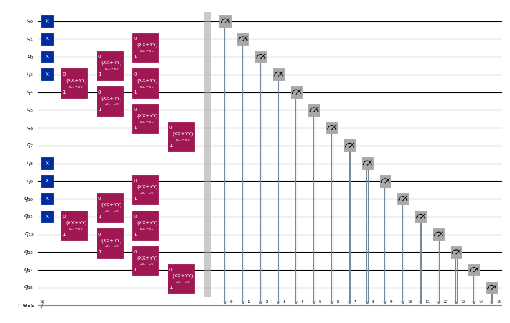
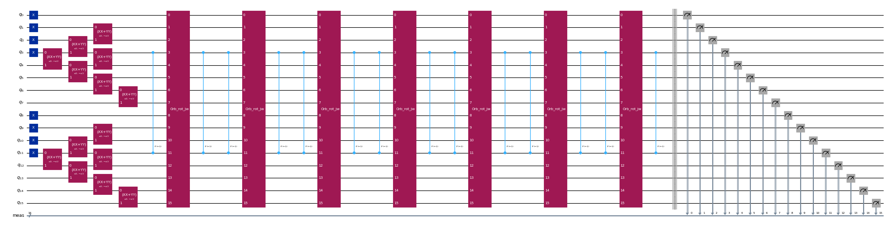
Als Nächstes erzeugen mir d Schaltkreise zur Erzeugung vun de Krylov-Basiszuständ. Für jede Spin-Spezies isch dr Anfangszustand $\ket{\psi_0}$ durch d Superposition aller mögliche Anregunge vun de drei Elektronen, die dem Fermi-Niveau am nächste sind, in d 4 nächste leere Mode gegebe, usgehend vum Zustand $|00\cdots 0011 \cdots 11\rangle$, und wird durch d Anwendung vun siebe XXPlusYYGates realisiert. D zeitentwickelte Zuständ werde durch sukzessive Anwendunge vun emm Trotter-Schritt zweiter Ordnung erzeugt.

Für e detailliertere Beschreibung vun dem Modell und wie d Schaltkreise entworfe worde sind, luag "Quantum-Centric Algorithm for Sample-Based Krylov Diagonalization".

from typing import Sequence

import ffsim
import scipy
from qiskit import QuantumCircuit, QuantumRegister
from qiskit.circuit import CircuitInstruction, Qubit
from qiskit.circuit.library import CPhaseGate, XGate, XXPlusYYGate

def prepare_initial_state(qubits: Sequence[Qubit], norb: int, nocc: int):
    """Prepare initial state."""
    x_gate = XGate()
    rot = XXPlusYYGate(0.5 * np.pi, -0.5 * np.pi)
    for i in range(nocc):
        yield CircuitInstruction(x_gate, [qubits[i]])
        yield CircuitInstruction(x_gate, [qubits[norb + i]])
    for i in range(3):
        for j in range(nocc - i - 1, nocc + i, 2):
            yield CircuitInstruction(rot, [qubits[j], qubits[j + 1]])
            yield CircuitInstruction(
                rot, [qubits[norb + j], qubits[norb + j + 1]]
            )
    yield CircuitInstruction(rot, [qubits[j + 1], qubits[j + 2]])
    yield CircuitInstruction(
        rot, [qubits[norb + j + 1], qubits[norb + j + 2]]
    )

def trotter_step(
    qubits: Sequence[Qubit],
    time_step: float,
    one_body_evolution: np.ndarray,
    h2e: np.ndarray,
    impurity_index: int,
    norb: int,
):
    """A Trotter step."""
    # Assume the two-body interaction is just the on-site interaction of the impurity
    onsite = h2e[
        impurity_index, impurity_index, impurity_index, impurity_index
    ]
    # Two-body evolution for half the time
    yield CircuitInstruction(
        CPhaseGate(-0.5 * time_step * onsite),
        [qubits[impurity_index], qubits[norb + impurity_index]],
    )
    # One-body evolution for the full time
    yield CircuitInstruction(
        ffsim.qiskit.OrbitalRotationJW(norb, one_body_evolution), qubits
    )
    # Two-body evolution for half the time
    yield CircuitInstruction(
        CPhaseGate(-0.5 * time_step * onsite),
        [qubits[impurity_index], qubits[norb + impurity_index]],
    )

# Time step
time_step = 0.2
# Number of Krylov basis states
krylov_dim = 8

# Initialize circuit
qubits = QuantumRegister(2 * norb, name="q")
circuit = QuantumCircuit(qubits)

# Generate initial state
for instruction in prepare_initial_state(qubits, norb=norb, nocc=norb // 2):
    circuit.append(instruction)
circuit.measure_all()

# Create list of circuits, starting with the initial state circuit
circuits = [circuit.copy()]

# Add time evolution circuits to the list
one_body_evolution = scipy.linalg.expm(-1j * time_step * h1e_momentum)
for i in range(krylov_dim - 1):
    # Remove measurements
    circuit.remove_final_measurements()
    # Append another Trotter step
    for instruction in trotter_step(
        qubits,
        time_step,
        one_body_evolution,
        h2e_momentum,
        impurity_index,
        norb,
    ):
        circuit.append(instruction)
    # Measure qubits
    circuit.measure_all()
    # Add a copy of the circuit to the list
    circuits.append(circuit.copy())

circuits[0].draw("mpl", scale=0.4, fold=-1)

circuits[-1].draw("mpl", scale=0.4, fold=-1)

Schritt 2: Problem für d Quantenausführung optimiere

Nachdem mir d Schaltkreise erstellt hän, köne mir sie für e Ziel-Hardware optimiere. Mir wähle d am wenigste ausgelastete QPU mit mindestens 127 Qubits. Weitere Informationen findet mr in dr Qiskit IBM® Runtime-Dokumentation.

from qiskit_ibm_runtime import QiskitRuntimeService

service = QiskitRuntimeService()
backend = service.least_busy(
    operational=True, simulator=False, min_num_qubits=127
)
print(f"Using backend {backend.name}")

Using backend ibm_fez

Jetzt verwende mir Qiskit, um d Schaltkreise für s Ziel-Backend z transpiliere.

from qiskit.transpiler import generate_preset_pass_manager

pass_manager = generate_preset_pass_manager(
    optimization_level=3, backend=backend
)
isa_circuits = pass_manager.run(circuits)

Schritt 3: Ausführung mit Qiskit-Primitiven

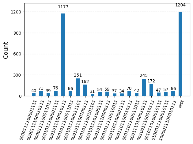
Nachdem mir d Schaltkreise für d Hardware-Ausführung optimiert hän, sind mir bereit, sie uf dr Ziel-Hardware auszuführe und Stichproben für d Grundzustandsenergieschätzung z sammle. Nachdem mir d Sampler-Primitive verwendet hän, um Bitfolge aus jedem Schaltkreis z zie, kombiniere mir alle Ergebnisse in emm einzelne Zähler-Wörterbuch und zeiche d 20 am häufigste gezogte Bitfolge uf.

from qiskit.visualization import plot_histogram
from qiskit_ibm_runtime import SamplerV2 as Sampler

# Sample from the circuits
sampler = Sampler(backend)
job = sampler.run(isa_circuits, shots=500)

from qiskit.primitives import BitArray

# Combine the counts from the individual Trotter circuits
bit_array = BitArray.concatenate_shots(
    [result.data.meas for result in job.result()]
)

plot_histogram(bit_array.get_counts(), number_to_keep=20)

Schritt 4: Nachbearbeitung und Rückgabe vum Ergebnis im gewünschte klassische Format

Jetzt führe mir dr SQD-Algorithmus mit dr Funktion diagonalize_fermionic_hamiltonian aus. Erläuterunge zu de Argumente vun dere Funktion findet mr in dr API-Dokumentation.

from qiskit_addon_sqd.fermion import (
    SCIResult,
    diagonalize_fermionic_hamiltonian,
)

# List to capture intermediate results
result_history = []

def callback(results: list[SCIResult]):
    result_history.append(results)
    iteration = len(result_history)
    print(f"Iteration {iteration}")
    for i, result in enumerate(results):
        print(f"\tSubsample {i}")
        print(f"\t\tEnergy: {result.energy}")
        print(
            f"\t\tSubspace dimension: {np.prod(result.sci_state.amplitudes.shape)}"
        )

rng = np.random.default_rng(24)
result = diagonalize_fermionic_hamiltonian(
    h1e_momentum,
    h2e_momentum,
    bit_array,
    samples_per_batch=100,
    norb=norb,
    nelec=nelec,
    num_batches=3,
    max_iterations=5,
    symmetrize_spin=True,
    callback=callback,
    seed=rng,
)

Iteration 1
	Subsample 0
		Energy: -28.61321893815165
		Subspace dimension: 10609
	Subsample 1
		Energy: -28.628985564542244
		Subspace dimension: 13924
	Subsample 2
		Energy: -28.620151775558114
		Subspace dimension: 10404
Iteration 2
	Subsample 0
		Energy: -28.656893066053115
		Subspace dimension: 34225
	Subsample 1
		Energy: -28.65277622004119
		Subspace dimension: 38416
	Subsample 2
		Energy: -28.670856034959165
		Subspace dimension: 39601
Iteration 3
	Subsample 0
		Energy: -28.684787675404362
		Subspace dimension: 42436
	Subsample 1
		Energy: -28.676984757118426
		Subspace dimension: 50176
	Subsample 2
		Energy: -28.671581704249885
		Subspace dimension: 40804
Iteration 4
	Subsample 0
		Energy: -28.6859683054753
		Subspace dimension: 47961
	Subsample 1
		Energy: -28.69418206537316
		Subspace dimension: 51529
	Subsample 2
		Energy: -28.686083516445752
		Subspace dimension: 51529
Iteration 5
	Subsample 0
		Energy: -28.694665630711178
		Subspace dimension: 50625
	Subsample 1
		Energy: -28.69505984237118
		Subspace dimension: 47524
	Subsample 2
		Energy: -28.6942873883992
		Subspace dimension: 48841

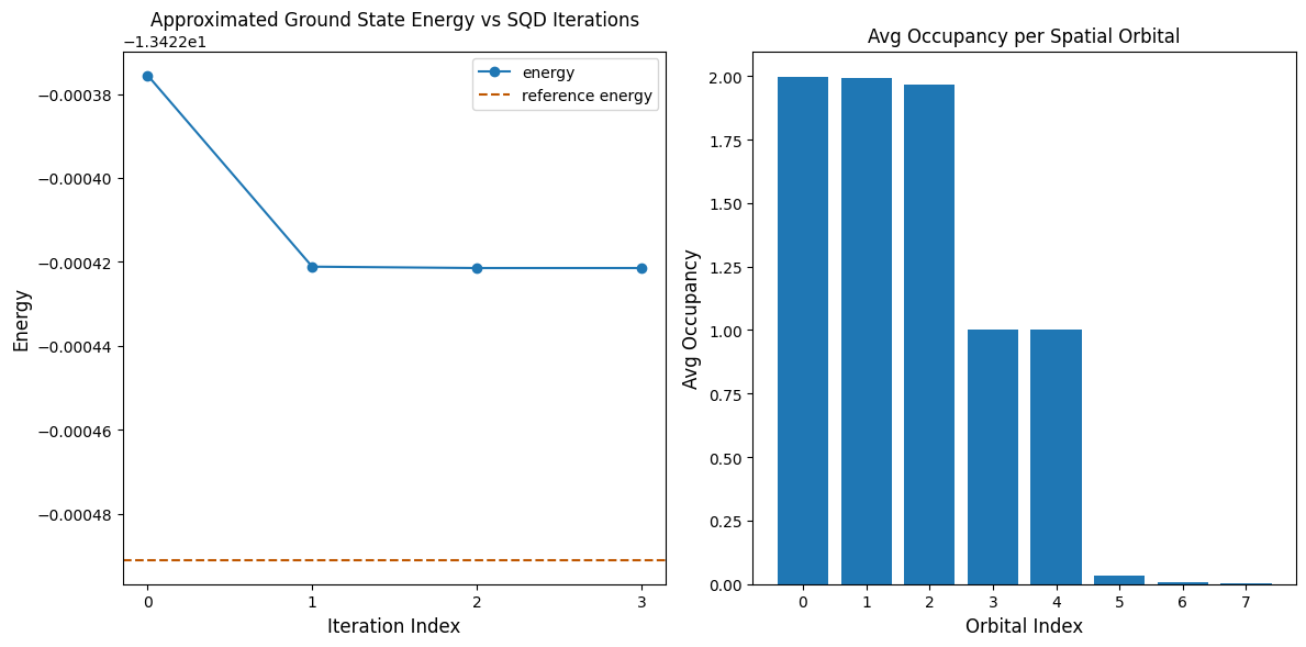
D folgende Code-Zell zeicht d Ergebnisse uf. D erste Grafik zeigt d berechnete Energie als Funktion vun dr Anzahl dr Konfigurationswiederherstellungsiterationen, und d zweite Grafik zeigt d durchschnittliche Besetzung vun jedem räumliche Orbital nach dr letzte Iteration. Für d Referenzenergie verwende mir d Ergebnisse vun enere DMRG-Berechnung, die separat durchgeführt worde isch.

import matplotlib.pyplot as plt

dmrg_energy = -28.70659686

min_es = [
    min(result, key=lambda res: res.energy).energy
    for result in result_history
]
min_id, min_e = min(enumerate(min_es), key=lambda x: x[1])

# Data for energies plot
x1 = range(len(result_history))

# Data for avg spatial orbital occupancy
y2 = np.sum(result.orbital_occupancies, axis=0)
x2 = range(len(y2))

fig, axs = plt.subplots(1, 2, figsize=(12, 6))

# Plot energies
axs[0].plot(x1, min_es, label="energy", marker="o")
axs[0].set_xticks(x1)
axs[0].set_xticklabels(x1)
axs[0].axhline(
    y=dmrg_energy, color="#BF5700", linestyle="--", label="DMRG energy"
)
axs[0].set_title("Approximated Ground State Energy vs SQD Iterations")
axs[0].set_xlabel("Iteration Index", fontdict={"fontsize": 12})
axs[0].set_ylabel("Energy", fontdict={"fontsize": 12})
axs[0].legend()

# Plot orbital occupancy
axs[1].bar(x2, y2, width=0.8)
axs[1].set_xticks(x2)
axs[1].set_xticklabels(x2)
axs[1].set_title("Avg Occupancy per Spatial Orbital")
axs[1].set_xlabel("Orbital Index", fontdict={"fontsize": 12})
axs[1].set_ylabel("Avg Occupancy", fontdict={"fontsize": 12})

print(f"Reference (DMRG) energy: {dmrg_energy:.5f}")
print(f"SQD energy: {min_e:.5f}")
print(f"Absolute error: {abs(min_e - dmrg_energy):.5f}")
plt.tight_layout()
plt.show()

Reference (DMRG) energy: -28.70660
SQD energy: -28.69506
Absolute error: 0.01154

Verifizierung vun dr Energie

D vun SQD zurückgegebene Energie isch garantiert e obere Schranke für d wahre Grundzustandsenergie. Dr Wert vun dr Energie ka verifiziert werde, da SQD au d Koeffiziente vum Zustandsvektor zurückgibt, dr dr Grundzustand approximiert. Mr köne d Energie aus dem Zustandsvektor unter Verwendung vun seine 1- und 2-Teilchen-reduzierte Dichtematrize berechne, wie in dr folgende Code-Zell demonstriert wird.

rdm1 = result.sci_state.rdm(rank=1, spin_summed=True)
rdm2 = result.sci_state.rdm(rank=2, spin_summed=True)

energy = np.sum(h1e_momentum * rdm1) + 0.5 * np.sum(h2e_momentum * rdm2)

print(f"Recomputed energy: {energy:.5f}")

Recomputed energy: -28.69506

Referenzen

• Quantum-Centric Algorithm for Sample-Based Krylov Diagonalization (SKQD paper)
• Chemistry Beyond Exact Solutions on a Quantum-Centric Supercomputer (SQD paper)
• Diagonalization of large many-body Hamiltonians on a quantum processor (KQD paper)